David Doolette has written a blog post “GRADIENT FACTORS IN A POST-DEEP STOPS WORLD” on the GUE blog that has caught some attention on the inter webs. He summarises the state of affairs about the current sentiment against too excessive deep stops, a trend that got momentum in the wake of the NEDU study.
It’s a nice summary but for those who followed the debates about this there are not too many news except in the last paragraph where he describes his personal take away: He says that newer results indicate that the increase in allowed over-pressures with depth (in the Bühlmann model expressed by the fact that the b-parameters are smaller than one and thus the M-value grows faster than the ambient pressure) is doubtful and that in fact the algorithms used by the Navy have the allowed over-pressure independent of depth, i.e. an effective b=1 for all compartments.
As with standard dive computers you are not at liberty to change the a and b parameters of your deco model. Rather the tuneable parameters are usually the gradient factors. So he proposes to set
\(GFlow = b GFhigh\)citing 0.83 being an average b parameter amongst tissues and thus justifying his personal choice of gradient factors to be 70/85 saying “Although the algebra is not exact, this roughly counteracts the slope of the “b” values.”
This caught my attention as many divers lack a good motivation for some specific setting of their gradient factors (besides quoting that “they always felt good with these settings” and thus ignoring that this is as best subjective anecdotal evidence for a statement the would need a much higher number of tests under controlled circumstances to have any significance.
We could add this as a feature to Subsurface where you could turn on “Doolette’s rule” and then your GFlow would automatically be set as 0.83 of your GFhigh (we could even use the actual b value for the compartment and make the GFlow depend on the compartment). Of course, since we have access to the source code, we could directly set the all the b’s to 1 by hand and get rid of the gradient factors in that mode entirely. That might involve also modifying the a’s (as the now depth independent M-value) which made me worry that I might be pulling numbers out of thin air which when implemented might cause other divers to actually use them in their diving while being without any empirical testing, something I wouldn’t like to be responsible for.
So, rather being the theoretical diver, I fired off mathematica to better understand the “non-exact algebra” and to see if it could be improved. Turns out “non-exact” is somewhat of a euphemism.
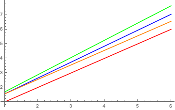
Of course, how bad this approximation is depends on the depth at which GFlow applies (i.e. the first stop depth) but from the plot it is clear that a constant M-value corresponds to smaller and smaller GFlow (as a fraction between the red and green line).
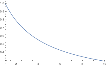
As you can see, for somewhat greater fist stop depths (corresponding to deeper and/or longer dives), to keep a depth independent M-value one needs such a small GFlow that I would consider this to be very well in deep stop territory, opposed to what the blog post started out with.
If you want to play around with the numbers yourself, here is the mathematica notebook.
I don’t think you want to look at “a” M-value line for this: you should plot all 16 (17). Because the slopes are different, I don’t believe the single green line gives you the full picture. Much of the rationale behind GF Lo in the first place is that the slope is much steeper for fast TCs, what you’re plotting is losing that dimension of it all.
I agree that this is missing. My plot shows only the tissue for which the assumption 1/b=0.83 is best. The situation worsens for the other tissues.