Decompression – The Theoretical Diver

Rating decompression

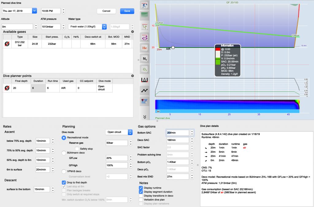
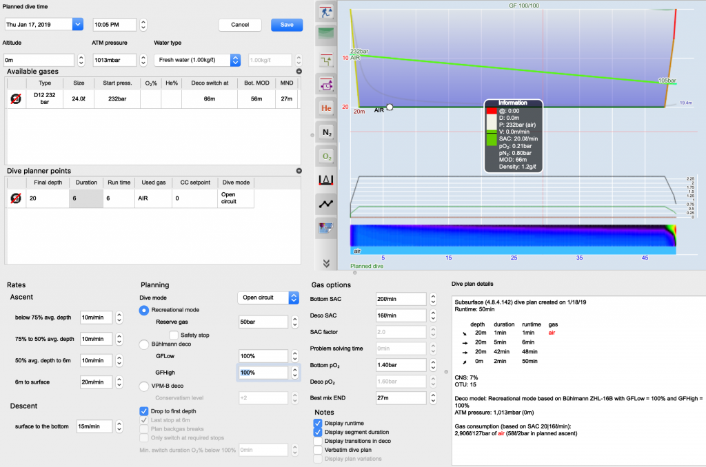
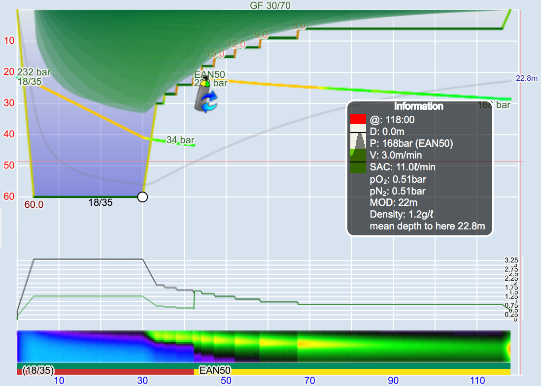
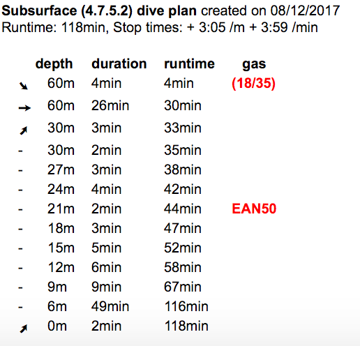
How good was the deco of my dive? For those of us who strive to improve their diving this is a valid question to find ways to optimise how we get out of the water. In Subsurface, for example, we give various information including the individual tissues’ ceilings as well as the heat-map.

Recently, on ScubaBoard, I learned about a new product on the market: O’Dive, the first connected sensor for personalised dives. It consists of Bluetooth connected ultrasound Doppler sensor together with an app on your mobile phone. The user has to upload the profile data of the dive to the Subsurface cloud from where the app downloads it and connects it with the Doppler data (for this, it asks for your Subsurface username and password?!?, the first place where you might ask if this is 100% thought through). Then it displays you a rating (in percent) for your deco and offers ways to improve it.

That sounds interesting. The somewhat ambitious price tag (about 1000 Euros for the sensor plus 1,50 Euro per dive analysed), however, prevented me from just buying it to take it for a test. And since it’s a commercial device, they don’t exactly say what they are doing internally. But in there information material they give references to scientific publications, mainly of one research group in southern France.

A fraction is to conference proceedings and articles in very specialised journals that neither my university’s library nor the Rubicon Archive not SciHub have access to, but a few of the papers I could get hold of. One of those is “A new biophysical decompression model for estimating the risk of articular bends during and after decompression” by J. Hugon, J.-C. Rostain, and B. Gardette.

That one is clearly in the tradition of Yount’s VPM-B model (using several of the bubble formulas that I have talked about in previous posts). They use a two tissue model (fitting diffusion parameters from dive data) and find an exponential dependence of the risk of decompression on the free gas in one of the tissues:

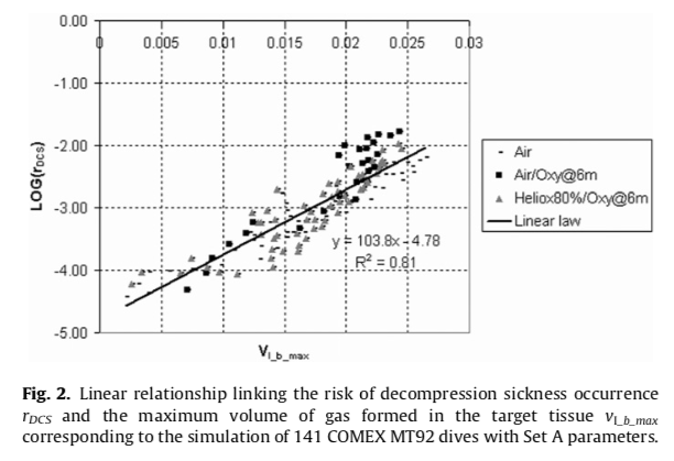
Note, however, that the “risk of decompression sickness” is not directly measured but is simply calculated from the

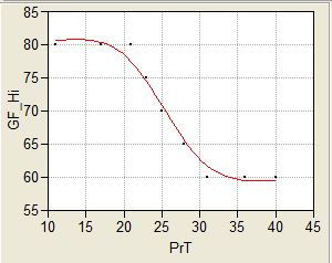
\(PrT = P\sqrt t\)

paramour (P is the ambient pressure in bar during the dive while t is the dive time in minutes, i.e. a characterisation of a dive profile compared to which a spherical cow in vacuum looks on spot, but this seems to be quite common, see also https://thetheoreticaldiver.org/wordpress/index.php/2019/06/16/setting-gradient-factors-based-on-published-probability-of-dcs/) using the expression

\(r_{DCS} = 4.07 PrT^{4.14}.\)

which apparently was found in some COMEX study. Hmm, I am not convinced Mr. President.

The second reference I could get hold of are slides from a conference presentation by Julien Hugon titled “A stress index to enhance DVS risk assessment for both air and mixed gas exposures” which sounds exactly like what the O’Dive claims to do.

There, it is proposed to compute an index

\( I= \frac{\beta (PrT-PrT^*)}{T^{0.3}} . \)

Here PrT=12 bar sqrt(min), T the total ascent time and beta depends on the gas breathed: 1 for air, 0.8 for nitrox and 0.3 for trimix (hmm again, that sounds quite discontinuous). As you might notice, what does not go into this index is at which depths you spend your ascent time while PrT keeps growing with time indefinitely (i.e. there is no saturation ever).

This index is then corrected according to a Doppler count (which is measured by a grade from 0 to 5):

Index correction according to Hugon teal

This corrected index is then supposed to be a good predictor for the probability of DCS.

I am not saying that this is really what is going on in the app and the device, these are only speculations. But compared to 1000 Euro plus 1,50 Euro per dive, looking at ceilings and heat map in Subsurface sounds like quite good value for money to me.de

Why are tissues independent?

This is the second instalment in a series of posts that are inspired by my reading about the SAUL deco model. Paradoxically, I want to report on something that I realised while reading the articles about that model even though Saul Goldmann, SAUL’s inventor, kindof comes to the opposite conclusion.

For the Bühlmann model, I have argued before that the different tissue half times are not really parameters of the model: If you have a tissue in contact with an environment (be it breathing gas or blood) it is pretty natural that gas diffuses between the environment and the tissue with a rate that is proportional to the difference of partial pressures

\(\dot p_i = d_i (p_a – p_i)\).

Here pi is the partial pressure in tissue number i, pa is the ambient partial pressure and di is the diffusion constant (essentially ln(2) divided by the half-time) of that tissue. This is the differential equation that governs all on- and off-gassing of tissues. To complete the Bühlmann model, one only has to specify a maximal tissue partial pressure in relation to the ambient pressure (or better a minimal ambient total pressure for a given tissue partial pressure) for which Bühlmann assumes an affine relation, i.e.

\(p_a \ge b_i (p_i – a_i).\)

It is important that the coefficients ai and bi for the tissue number i are really parameters of the model that need to be determined empirically (and for which there are tables). The diffusion constants (and thus tissue half-times), however, are not.

You only need to make sure you satisfy the inequality for all possible tissues, that is for all possible half-times. To do so, you try to do the calculation for all relevant time scales. In the case of (non-saturation) diving, the relevant times go from a few minutes (the shortest relevant time scale of ascents and descents) to a few hours.

Of course, you cannot calculate for all possible times. But you make sure, you cover this range of times with many representative times. And a little further thought reveals that you should spread those representative times geometrically (so also the range of diffusion constants is covered geometrically).

To sum up, you need to know the a’s and the b’s but for the d’s, you essentially cover all possible values. It is important, that for this result we had to know nothing about actual tissues like bones, nerves, muscles or whatever of the human body, since all that is relevant that they have some diffusion constant in the relevant range.

So far, this was all old news.

Today, I want to look at the question, why we can get away with treating all these tissues independently. Why does tissue number i only exchange inert gas with the blood stream or the breathing gas and not with all the other tissues?

In the Bühlmann model, each tissue exchanges inert gas directly with the blood stream.

Maybe, this assumption is unrealistic and we should better consider a model that looks like this:

Every tissue potentially exchanges gas with all the other tissues.

Maybe, we should allow tissues i and j to exchange gas directly. This would be described by a new diffusion constant cij (non-negative and possibly zero if the tissues are not connected) and the new differential equation would look like

\(\dot p_i = d_i (p_a – p_i)+\sum_{j\ne i} c_{ij}(p_j – p_i)\).

In order for no gas to get lost, we would need cij to equal cji. To simplify this, we could assemble the different partial pressure pi into a vector p, the diffusion constants di into a vector d and the new diffusion constants cij into a symmetric matrix C.

If you have only a little experience with ODE’s, you realise that this equation is a linear inhomogeneous ODE and can be written in the form

\(\dot p = Ap + p_a d\)

where the matrix A has components

\(a_{ij} = -c_{ij} + \sum_k c_{ik} \delta_{ij} – \delta_{ij} d_i.\)

A quick inspection shows that A is symmetric and negative definite (if all di are positive).

The key observation is that we can diagonalise A as

\(A= U^{-1}DU\)

where D is diagonal with all negative eigenvalues. Then the above differential equation reads

\({d\over dt}(Up) = D (Up) + p_a Ud.\)

But thanks to D being diagonal, we can view this as a new vector Up of tissue partial pressures that obey the original Bühlmann differential equation! So up to taking linear combinations, the Bühlmann model already covers the case of tissues directly exchanging inert gases. Allowing for this apparent generalisation of the model can be converted by simply a change of basis.

So, if we say, that the modelled tissues are not really corresponding to actual tissues (as we already did above) but allow the interpretation that they might be linear combinations of actual tissues, then the Bühlmann model already covers (as long as we cover all possible diffusion constants which we do) the case of inter-tissue gas exchange. It is not a special case in this wider class of modes with interconnected tissues but it is already the generic case.

Let me close with a consistency check: At content depth, pa is constant. In this case, Up converges saturates to

\((Up)_i \to \frac{(Ud)_i}{\lambda_i}p_a.\)

or in matrix notation

\(p\to U^{-1}D^{-1}Ud p_a = A^{-1}dp_a.\)

But a quick calculation shows that if v is the vector that has ones in all components

\(Av = d\)

and thus finally

\(p_i\to A^{-1}dp_a = vp_a\)

and hence indeed all tissue partial pressures approach the ambient partial pressure.

Fraedrich follow-up

Here is a second guest post by Doug Fraedrich on how to select gradient factors:

For this next phase of the analysis, we will probe the GF-Hi vs PrT issue with other suitable data sources other than the Van Liew and Flynn model and look into the GF-Lo question without direct reliance on the 2011 NEDU Deep Stop experiment.

There are several suggested methodologies in the literature for the validation of models in general (Reference 1) and dive computers in particular (Reference 2.) The method I used above is similar to one suggested in Reference 2, of comparing the results of a commercial dive computer to one of the US Navy probabilistic models (which are essentially least-squares fit to many DCS observations); in this case the Van Liew and Flynn “StandAir” model was used. Another possible approach suggested in Reference 2 is to compare the unit under test directly to well-validated Navy dive tables, i.e. VVAL-79 (Note that VVAL-79 is an updated version of VVAL-18, which was necessitated by an unacceptably high incidence of DCS using VVAL-18.) Denoble suggests a similar but more general approach of comparison to so-called “primary models” which include VVAL-79 and also the Canadian DCIEM tables (Reference 3). Denoble defines “Primary Models” as those that have been extensively and methodically tested with man-trial data. For the remainder of this article, we will limit our analysis to using Primary Models. The validation of commercial dive computer algorithms is in its infancy, so it is instructive to use different sound methodologies and different “gold standards” to get a sense of the uncertainty in results. As a community, we can make it our goal to continually refine our methods and use new data as it becomes available to reduce this uncertainty over time.

In this new cross-validation study, the ZHL-16C model was iteratively run with different values of GF-Lo and GF-Hi to match the results VVAL-79 and DCIEM Tables.

The results are shown in the Figure 1 below.

The diagonal nature of the VVAL-79 results reflects that both GF-Lo and GF-Hi are indicated to decrease with increasing PrT; this not surprising since the Van Liew and Flynn data mentioned above also was used in the Navy’s model development and validation process. Note that the results for the DCIEM tables do not exhibit this behavior.

In order to add more information to this analysis, we will consider a third model, SAUL, which is an update of the original Kidd-Stubbs DCIEM serial model and would certainly meet the Denoble criteria of a “Primary Model.” It has been tested by three datasets of man-dives with P-DCS statistics: a core dataset of 733 dives (Reference 4) and two secondary datasets, DSAT (1437 man-dives) and the NEDU 2011 Deep-stop dataset (390 man-dives.) A full dive-planner is not openly available for this model, but an online version is available that handles no-decompression dives, and estimates P-DCS of a specified dive profile assuming a 3 minute safety stop.

For selected combinations of GF-Lo and GF-Hi, the ZHL-16C model is run iteratively with varying values of depth and bottom time to yield a 3 minute shallow stop. The SAUL dive planner is then run with those depth and bottom time values and the estimated P-DCS is computed. This P-DCS is plotted as a function of GF-Lo and GF-Hi, Figure 2. Unfortunately, for a given value of GF-Hi, only a narrow range of GF-Lo meet the criteria of mandating a 3 minute shallow stop (clearly illustrated in Figure below.) So these new results do NOT inform the GF-Lo debate nor the GF-Hi vs PrT issue. It does quantify P-DCS for a diagonal swath of GF values; which is a good start. So if your risk tolerance is say 0.25%, you would want to set GF-Hi between 80 and 85.

It is worth noting that these three primary models are not only well-tested with man-trial data, they are based on differentdatasets. So any conclusion based on areas of common agreement amongst these models can be considered as having a fairly low uncertainty.

To try to summarize where I think we are based on these data sources using the 3 primary models VVAL-79 DCIEM and SAUL, and supplementing with references to the data-based statistical models from both Howie et al and Van Liew and Flynn (both based on large datasets of man-trial DCS data), see the results below, which are partitioned into a 2×2 matrix:

	Low PrT Dives/Non-Deco Dives	High PrT Dives/Deco Dives
GF-Hi	All 5 sources agree on a range of 80-90	VVAL-79 and Van Liew and Flynn indicate 60-70; DCIEM shows 80-85. SAUL and Howie are silent
GF-Lo	VVAL-79 and DCIEM agree on a range of 75-85, while the other 3 sources are “silent” or non-informative	VVAL-79 indicate 60-70; DCIEM shows 75-85. SAUL, Howie and Van Liew and Flynn are silent

For Low PrT dives, I would consider the recommendations for GF-Hi to be fairly conclusive. A little less so for GF-Lo, but there is an extensive man-dive database for these types of dives to back it up. For High PrT dives, we see the two main Primary models, VVAL-79 and DCIEM result in recommended ranges that do not overlap; so this is an area of future focus. Recommendations for GF-Lo for High PrT dives are the most uncertain. Several potential ways-ahead come mind. The full SAUL model could be executed to estimate P-DCS of dive profiles computed by ZHL-16C over the entire range of gradient factors. Or potentially, the DAN Project Dive Exploration observational database (Reference 5) could be mined to focus at high PrT dives, and convert reported dive profiles to equivalent ZHL-16C results with whatever GF’s are needed to match the profiles. The issue here may be to adequately address potential underreporting of dives where no DCS was present, and thus attempting to ensure the resultant P-DCS statistics are unbiased. Clearly more work is needed here.

References:

Fraedrich D and Goldberg A “A methodological framework for the validation of predictive simulations” European Journal of Operational Research, 124(1):55-62 · July 2000
Doolette DJ, Gault KA, Gerth WA, Murphy FG. US Navy Dive Computer Validation. In: Blogg SL, Lang MA, Møllerløken A, editors Proceedings of Validation of Dive Computers Workshop 2011 Aug 24 Gdansk. Trondheim: Norwegian University of Science and Technology; 2012. p. 51–62.
Denoble PJ. Conservative diving: calculating and mitigating the risk of DCS. Alert Diver 2013; 29(3): 46-9.
Goldman S, A new class of biophysical models for predicting the probability of decompression sickness in SCUBA diving. Journal of Applied Physiology, 2007. On-line dive planner at: http://moderndecompression.com/?page_id=493

https://www.diversalertnetwork.org/research/projects/pde/

Setting Gradient Factors based on published probability of DCS

This is a contributed post by Doug Fraedrich in which he reports on a recent paper by him and which is also mentioned in Doolette’s blog post I just commented on.

Recently I published a methodology on how to set conservatism factors on commercial dive computers based on published probability of decompression sickness (DCS) data and statistical summaries/models thereof, (Reference 1.) That paper described the general methodology on how to adjust the conservatism of several different algorithms; this note will focus specifically on setting gradient factor levels for the Bühlmann ZHL-16C algorithm.

The basic methodology is to use the output of probabilistic models from the literature that were derived from many well-documented experimental man-trials of known dive profiles. Then pick a probability of DCS isopleth curve and use those to set gradient factors (or conservatism factors) such that the algorithm will output the No-stop time or total decompression time (TDT) specified by that isopleth. This was done for three metrics: no-stop times for short recreational dives profiles, total decompression time for longer/deeper decompression dives and “first stop depth” for decompression dives. There were no probabilistic models for first stop depths/decompression profiles, so for this metric, we used data from a NEDU controlled experiment, which compared P_DCSoutcomes of dives of the same depth, bottom time and same TDT but with different stop profiles (Reference 2.) This NEDU study was performed specifically to assess the effect of deep versus shallow profiles as dictated by dual-phase vs tissue-loading algorithms.

So now to apply the methodology from that paper to the task of setting Gradient Factor levels for the Bühlmann ZHL-16C algorithm. From previous publications on the topic of gradient factors, we know that the value GF-Hi mainly affects total decompression time and GF-Lo affects the depth of the first stop. For GF-Hi, we will use the probabilistic model from a new study on No Stop Times by Howie et al. (Reference 3.) Using their criteria of 0.1 % serious DCS, we pick several point-pairs of depth and No-stop time and iteratively run theBühlmann ZHL-16C algorithm (specifically MultiDeco version 4.12)with different values of GF-Hi and match at what level the algorithm allows for a direct ascent at each individual depth-bottom time pair. The corresponding value of GF-Hi is 80.

As mentioned above, for GF-Lo, we use the US Navy NEDU study on deep stops, Reference 2. In the NEDU study, the maximum depth was 170 fsw, the bottom time was 30 minutes, the ascent rate was 30 fsw/min and the TDT for both profiles was 180 minutes. The group of divers who started their first stop at 40 fsw (for 9 minutes) had significantly lower P_DCS(P= 0.0489 one-sided, Fisher Exact Test) than the group that stopped first at 70 fsw (for 12 minutes). Since there is not sufficient information to know exactly where between the two tested depths is optimal, this test case used the two depths as a maximum and minimum for the first stop criterion. For that dive profile, MultiDeco was iteratively run varying GF-Lo to see which levels of GF-Lo yield the two limiting first stop depths. This procedure indicates that GF-Lo should be higher than 55 (this was previously reported in Reference 1.) If you pick the mid-point of the two first stop depths between those profiles (assuming the optimal point is somewhere in the middle and not at either extreme) the resulted in GF-Lo being on the order of 70.

Of course, the above setting for GF-Hi was based on no-decompression dives which had a relatively low value of PrT of ~10-12 (Pressure Root Time is an indicator of the severity of the dive exposure where P = pressure in bar, T = dive time in minutes, Reference 4.)We know from Reference 4 that historically, the incidence of DCS is significantly higher for dives with a PrT > 25 and we know from Reference 1 that the required value of GF-Hi for ZHL-16C needs to decrease as the PrT of the dives increases. So to set GF-Hi for higher PrT decompression dives, we re-visited methods and models presented by Van Liew and Flynn, where they were specifically assessing the suitability of the US Navy’s decompression schedule (used at that time) by fitting data on single-level, non-repetitive, nitrogen-oxygen dives from the US Navy Decompression Database to a logistic regression that resulted in P_DCSisopleths as a function of bottom time and TDT (Reference 5).We limited the domain of applicability of the current study to PRT< 40, so we used the “StandAir” Model which Van Liew andFlynn based ondata from standard air dives which had depths of less than 190 fsw and bottom times of less than 720 minutes. They assessed the StandAir statistical model to be reasonable except at the two depth extremes (nominally < 60 fsw and > 190 fsw). Van Liew and Flynn compared TDT required by the algorithm-under-test to the P_DCSisopleths from their statistical model, and found that the TDT required by the algorithm-under-test lay between the 2% and 3% P_DCSisopleths and thus deemed the algorithm acceptable for US Navy use. In the current study, we selected the 3% P_DCSisopleth as an initial standard of comparison as a compromise between managing DCS risk while not requiring excessive total decompression times. Note that in their analysis, they combined data from all dives that had the same depth and bottom time, thus their PDCS results are averaging over many different (non-optimal) decompression profiles.

The process here is similar to what was described above using the No Stop Data, only with the Deco dives, it was a trio of data values of: depth-bottom time-TDT (at the 3% PDCS isopleth curve.) MultiDeco was iteratively run to match TDT for the input values of Depth and bottom time. The value of GF-Hi was noted and plotted against the PrT of the dive profiles used. These results are summarized in Figure 1.

Note the curve in Figure 1 is of sigmoid shape: It is flat at both low and high levels of PrT with a transition in between. These results are based on dive profiles with observed DCS symptoms, and there are many more dives at the lower end of the PrT scale than the higher; so generally speaking the “error bars” start off small on the left side of the graph and get bigger as PrT increases. The point at which it levels out is considered somewhat uncertain.

To summarize:

GF-Lo is recommended to be >= 55
The recommended level of GF-Hi depends on the PrT of the dive, but is never greater than 80. It decreases with increasing PrT of the dive (to a point)
While the uncertainty at the low end (say PrT < 25) is low, it increases with PrT (i..e. more research is needed in this part of the domain.)

References:

Fraedrich DS, Validation of algorithms used in commercial off-the-shelf dive computers, Diving and Hyperbaric Medicine, V48 No 4 , 2018
Doolette DJ, Gerth WA, Gault KA. Redistribution of decompression stop time from shallow to deep stops increases incidence of decompression sickness in air decompression dives. NEDU TR 11-06, Panama City FL; 2011.
Howie, LE, Weber PW, Hada E, Vann RD, Denoble PJ, The probability and severity of decompression sickness, PLoS ONE 12(3): e0172665,2017
Balestra C. Dive computer use in recreational diving: Insights from the DAN-DSC database. In: Blogg SL, Lang MA, Møllerløken A, editors. Proceedings of validation of dive computers workshop. 2011 Aug 24 Gdansk. Trondheim: Norwegian University of Science and Technology; 2012. p. 99–102.
Van Liew HD, Flynn ET. A simple probabilistic model for standard air dives that is focused on total decompression time. Undersea Hyperb Med.2005;32:199–213.

Short comment on Doolette’s “GRADIENT FACTORS IN A POST-DEEP STOPS WORLD”

David Doolette has written a blog post “GRADIENT FACTORS IN A POST-DEEP STOPS WORLD” on the GUE blog that has caught some attention on the inter webs. He summarises the state of affairs about the current sentiment against too excessive deep stops, a trend that got momentum in the wake of the NEDU study.

It’s a nice summary but for those who followed the debates about this there are not too many news except in the last paragraph where he describes his personal take away: He says that newer results indicate that the increase in allowed over-pressures with depth (in the Bühlmann model expressed by the fact that the b-parameters are smaller than one and thus the M-value grows faster than the ambient pressure) is doubtful and that in fact the algorithms used by the Navy have the allowed over-pressure independent of depth, i.e. an effective b=1 for all compartments.

As with standard dive computers you are not at liberty to change the a and b parameters of your deco model. Rather the tuneable parameters are usually the gradient factors. So he proposes to set

\(GFlow = b GFhigh\)

citing 0.83 being an average b parameter amongst tissues and thus justifying his personal choice of gradient factors to be 70/85 saying “Although the algebra is not exact, this roughly counteracts the slope of the “b” values.”

This caught my attention as many divers lack a good motivation for some specific setting of their gradient factors (besides quoting that “they always felt good with these settings” and thus ignoring that this is as best subjective anecdotal evidence for a statement the would need a much higher number of tests under controlled circumstances to have any significance.

We could add this as a feature to Subsurface where you could turn on “Doolette’s rule” and then your GFlow would automatically be set as 0.83 of your GFhigh (we could even use the actual b value for the compartment and make the GFlow depend on the compartment). Of course, since we have access to the source code, we could directly set the all the b’s to 1 by hand and get rid of the gradient factors in that mode entirely. That might involve also modifying the a’s (as the now depth independent M-value) which made me worry that I might be pulling numbers out of thin air which when implemented might cause other divers to actually use them in their diving while being without any empirical testing, something I wouldn’t like to be responsible for.

So, rather being the theoretical diver, I fired off mathematica to better understand the “non-exact algebra” and to see if it could be improved. Turns out “non-exact” is somewhat of a euphemism.

Allowed over pressure: Green is 100/100 plain vanilla Bühlmann, blue 70/85 as of Doolette, orange is actually b=1 depth independent and red is ambient pressure. All numbers are bar.

Of course, how bad this approximation is depends on the depth at which GFlow applies (i.e. the first stop depth) but from the plot it is clear that a constant M-value corresponds to smaller and smaller GFlow (as a fraction between the red and green line).

Required GFlow/GFhigh for constant M-value as a function of ambient pressure (in bar) at first stop

As you can see, for somewhat greater fist stop depths (corresponding to deeper and/or longer dives), to keep a depth independent M-value one needs such a small GFlow that I would consider this to be very well in deep stop territory, opposed to what the blog post started out with.

If you want to play around with the numbers yourself, here is the mathematica notebook.

Intro to Bühlmann/GF by H&W

In my posts here at the theoretical diver, I usually assume that besides some mathematics and physics literacy (which allows me to use formulas) my readers already know about the workings at least of the Bühlmann model and its generalisation using gradient factors.

Of course, that assumption is not always justified and for some time I wanted to write a foundational post on these topics (maybe with some personal twist, let’s see) but I never got around doing that. There is my old text (in German) but that covers only the very basics and in particular it is very short on gradient factors.

Some consolation was that there are a number of such descriptions available on the inter-webs. But now, on the occasion of the Boot trade show, there is a new one written by Ralph Lembcke und Matthias Heinrichs of Heinrichs Weikamp, the manufacturer of OSTC dive computers (and friends of the blog), Matthias and Ralph are now the principal developers of the OSTC firmware. It has a broader audience (and is in German as well) in mind and thus does a good job using diagrams instead of formulas. I like it a lot and give a strong reading recommendation (even though I might phrase the justification for using smaller GFlow differently, and there is of course my private pet peeve of not thinking of tissue half times as part of the model)!

Update September 2020: Now also available in English.

NDL and Gradient Factors

There is an interesting discussion over at ScubaBoard how the non-decompression limit (NDL) is affected by the settings for gradient factors (GFlow and GFhigh), in particular which of the two is relevant. My initial reaction was: It’s clearly GFlow, as that sets the depth of the first stop and the criterion for NDL is that the (theoretical) first stop is at a depth of 0.

Others argued that it must be GFhigh as that applies, by definition, at the surface.

And indeed, in this limit (of the first stop is at the surface) the idea of gradient factors degenerates: In that limit, the rate of change of effective gradient factor as a function of depth diverges. So, like in the last post, there is an interesting point that involves taking limits.

What I had in mind is the implementation in Subsurface: As you can see, as long as there has not been a stop yet (because the ceiling is still above the surface), the effective gradient factor is GFlow. So, in a no decompression dive, you would think, you never see anything else.

But to show that in the recreational mode in the planner turned out so be quite hard: I had to play a lot with the parameters to find a dive where GFlow has any influence on the total dive time of a recreational dive (defined as a dive without mandatory stops and without running out of gas). Eventually I found one: For an air dive to 20m (with an ascent rate of 20m/min for the last segment, see below why this is important), you get a maximal run time of 49min with GF settings 20/100 while you can stay for 50min with GF settings of 100/100. But changing GFhigh has much stronger influence:

What did I miss? In the end, it’s the fine-print of the definition of “first stop depth” that I already talked about in an earlier post: The problem is that for real world dives there is no clear distinction between ascent and stop. So you need to come up with some definition which depth one wants to use to actually anchor GFlow. Subsurface uses the lowest ceiling encountered during the dive so far. But in particular for dives with very little (or none at all) deco obligation that is not exactly what others might consider the first stop depth. The difference is that the diver first need to get to that depth of the ceiling before the ceiling actually becomes a stop depth. And during that ascent, there is already off-gassing going on which can eliminate the ceiling during the time it takes the diver to get there.

As an example, you could have a first ceiling (which as I explained above is determined by GFlow) at say 1m of depth. But then, in this last meter of water, the effective gradient factor has to vary from GFlow to GFhigh. Given that we are talking about dives that are only marginally deco dives, it is likely that this first ceiling comes form a very fast tissue so it is likely that much of it goes away during the short time of ascent to that depth. Then, to find the NDL, the remaining question is if there is ceiling left below the surface. But then the GFlow is already anchored at 1m so for the surface it’s really GFhigh (and GFlow is no longer relevant as there is no ceiling left at 1m where it applies).

So the challenge to find a dive where GFlow makes any difference at all for the NDL was to produce a dive where there is something left of the initial ceiling at the time when the diver gets there in the marginal case of staying a little bit shorter not occurring any stops at all. So the dive must not be too deep (otherwise the ascent takes too long and there is a lot of on the way off-gassing). That’s why I had to increase the ascent rate.

So the upshot is: It is almost entirely GFhigh that sets the difference between a non-stop dive and a decompression stop dive. But if you stay a little bit longer the depth of your first stop (and also the duration) depends a lot on GFlow.

I should not end without pointing out that once more this discussion is quite academic: Gradient factors were invented for dives that have significant deco obligation to force deeper stops. Here, we are in the limit of recreational no-stop diving. So we are really not in the realm of gradient factors. And this manifests itself in the degeneracy of the model in the case of the ceiling being exactly at the surface that determines the NDL. But it was interesting anyway.

Can we calculate no-fly-times?

There are various recommendations how long one should not fly after surfacing from a dive. DAN has recently done a study where they did Doppler measurements on a plane and recommends an interval of 12 hours after a single dive and 24 hours after repetitive diving.

But one would think that it should be possible to use a decompression model that works well under water to compute such a time. So let’s do this in this post or at least compute a conservative estimate. To be specific, we will use the Buhlmann model. We do that calculation compartment by compartment and assume that when leaving the water, the tissue has the maximally allowed partial pressure for surfacing (i.e. this tissue was the guiding tissue for the final part of the ascent). Clearly, this is a conservative assumption. Then, according to the model

\(p_s = (p_i -a)b.\)

Here, ps is the surface pressure and a and b are the usual Bühlmann coefficients.

Then we do a surface interval (whose length we wish to determine in the end) during which the partial pressure decays exponentially:

\(p_i(t) = f_{N_2} p_s+ (p_i(0) – f_{N_2}p_s)e^{-\gamma t}\)

where f is the N2 fraction the the breathing gas (0.79 for air which we are probably breathing while waiting for the plane to board). Finally, we don’t want the cabin pressure to be less than the minimal ambient pressure that Dr. Bühlmann recommends. We want to parametrize the cabin pressure using the barometric formula which asserts (assuming constant temperature) that the pressure drops exponentially at height with decay constant that the pressure is 1/e at about hs=8500m above sea level. So, we set

\(e^{-h/hs} p_s= (p_i(t) -a)b.\)

This we can then solve for t. Actually, being conservative, we want to throw in gradient factors. Again, being conservative, we don’t further linearly extrapolate gradient factors, but will use GFhi everywhere on the surface. Plugging everything in (with the help of Mathematica and some manual massaging) we find

\(e^{\gamma t} = \frac{a GF/p_s + 1-f_{N_2} + GF(1/b -1)}{a GF/p_s – f_{N_2} +e^{-h/h_s}(1+GF(1/b-1))}.\)

Now, we have to plug in numbers. For the cabin pressure, according to Wikipedia, we will assume h=2400m for older aircrafts. The wait times (in hours) for the different compartments are then shown in this plot:

No-fly-times in hours for different compartments plotted against gradient factor. The labels are the tissue half-times in minutes.

You are supposed to see a number of things:

The waiting time depends strongly on which tissue we are dealing with. For reasonably large gradient factors, only the tissues with half-times of several hours contribute significant waiting times. Remember, for this calculation, we assumed the loading is at its maximal value when you get out of the water. For realistic sports/tec-diving scenarios (as opposed to saturation diving) that should be quite hard even on a weeklong liveaboard with at least five dives a day. If slightly faster tissues are leading, the inferred no-fly times are much shorter, probably shorter than the queue at check-in. I looked at some data from real dive trips where people got everything out of their booked liveaboard but they got nowhere close to exciting the slow tissues. In the Subsurface planner I had to do five consecutive 2-hour dives with less than two hour surface interval to see at least some ceiling for the 239 minute compartment. In the plots, this has the blue line and leads to a no-fly time of much less than 5 hours.
The plot ends on the left (small gradient factors) with diverging values. These divergences move to higher gradient factors when you increase the cabin pressurisation equivalent altitude (for example by assuming a loss of cabin pressure, remember this is when the oxygen masks are supposed to drop from the ceiling)
Same plot with 4500m of altitude

This comes about as the no-fly time becomes infinite or even complex as according to the Bühlmann-with-gradient-factors limit, your are not allowed to be at the ambient pressure at that altitude even when saturated with the nitrogen that you experience at sea level. We can compute this limiting altitude by solving
\(f_{N_2} p_s = e^{-h/h_s} p_s (GF/b-GF +1) + a GF /p_s\)
for the altitude via
\(e^{-h/h_s} = \frac{f- aGF/p_s}{GF/b -GF +1}.\)
This is shown here, the maximum altitude after waiting an infinite amount of time:

Maximal altitudes in meters for the different compartments as a function of the gradient factor.
All these calculations are for air (or nitrox underwater since all we used was the assumption that the nitrogen saturation is at the limit). In particular, in view of an earlier post (N2 vs. He, what’s the difference?) there should not be large differences.
You could try to repeat the same argument for VPM-B but according to that model, if you followed it during the ascent, the no fly time would always be infinite: The ascent is determined such that when you surface and stay at ambient pressure, you will just create the maximum amount of free gas that is barely allowed. So going to any altitude and lowering the ambient pressure further would release more free gas than allowed, no matter how long you waited. The only way out would be to produce fewer bubbles on the earlier ascent while still in the water, then you would have some reserves to go to altitude.

What are we supposed to conclude from this? One takeaway message is waiting for the recommended 24 hours is not totally off, in particular if there is a chance that your very slow tissues have loaded a significant amount of nitrogen.

On the other hand, for realistic dives, 24 hours is likely on the very conservative side. At least from the perspective of decompression theory. From this perspective it is a total mystery to my what kind of reasoning dive computers use to determine a no-fly time.

Apart from these model considerations, DCS symptoms often enough do not show up immediately after a dive but up to several hours later. And when you are in that situation that you find yourself with DCS symptoms (even those that would have occurred irrespective of flying or not) your chances for immediate proper treatment are probably much higher if you are not confined to an aircraft above the middle of the ocean. So even from that perspective it makes sense to wait a bit more to make sure you will not need a chamber in the next few hours.

PS: If you want to play around with the formulas, here is my Mathematica notebook.

VPM-B for real dives (or not)

The VPM-B model (of which I have described my understanding in previous posts) has a “derivation” in terms of bubble physics which I, as readers should have noticed, have some trouble to follow through completely as it is, to say the least, ad hoc and sketchy in places. I bet, only based on this derivation in prose plus formulas, nobody would be able to write a program to compute a VPM-B deco plan.

But we are lucky: There is a reference implementation in terms of a FORTRAN program. So, even though the VPM-B code in Subsurface is a complete rewrite (and solves many things algorithmically differently than the original code), we did a lot of testing to make sure that the plans we produce are identical to the plans computed using the FORTRAN program, even in places where we thought it makes little sense (like starting the ascent to the next stop when the ceiling depth equals the depth of the next stop rather than starting a bit earlier and making sure never to violate the ceiling during the ascent to the next stop (which is different since the ceiling goes up during the time it takes to get to the next stop). The latter is, at least to me, better motivated physically (“simply never violate the ceiling”) than basing the stop time on what happens at a different depth (namely the next stop depth) and we use the latter when computing Bühlmann schedules. But for VPM-B, we thought, given that we do not really understand the physics, we should not modify the model based on physics.

I have talked in the past about the Bühlmann model not being well defined to make all implementations come up with identical plans. In a sense, we are in a better situation with VPM-B, since there is the FORTRAN program which (at least for us) defines the model. But the problem is: This definition works only for the situation that you can compute with the FORTRAN program: You specify the bottom part of the dive and then let the program work out the ascent. Strictly speaking there is no definition for real dives: Dives where the distinction between bottom part and deco is blurred. But this is exactly what you have if you were to implement it in a dive computer or, as for Subsurface: Implement it in a dive log to show a ceiling for a logged dive (after all, Subsurface is mainly a divelog). For real dives, you cannot tell the exact point where bottom time ends and deco begins.

Unfortunately, the model depends on this: As explained in the VPM-B derivation post, one parameter that goes into the computation is the total deco time \(t_D\) (clearly that ends when you reach the surface, but where does it start?) but there are other parameters that you are supposed to evaluate at the beginning of the ascent like \(p_{1st ceiling}\) and the initial gradient for the Boyle compensation. All this depends on the time you call the end of bottom time and thus the computed ceilings also depend on that.

For Subsurface, we decided to take the point of time with the deepest ceiling (which, strictly speaking, is a circular definition but in practice is irrelevant) as the end of bottom time and base the ceiling computation in logbook mode on that. But that, to some degree, is arbitrary. And even for dives that we planned using VPM-B (and thus agree with the schedules computed by the FORTRAN program), applying this logic yields a slightly different ceiling. So it can appear that a VPM-B planned dive violates the VPM-B ceiling. But this is only due to the fact that the model is not really defined outside the planning situation.

Or put differently: You need to make arbitrary assumptions (not based on the depth profile and the gas you are breathing) to come up with a VPM-B ceiling. Which, at least for me, doesn’t strengthen my believe into this model.

PS: I am planning to be at the Boot dive show in Düsseldorf on Friday January 26th. If you happen to be there as well, please let me know and we can shake hands!

DIY on the fly

With the new version of Subsurface out today, I would like to point to a feature that was already there in 4.7.4, but which just got more usable: Computing deco variations in the planner.

This is motivated by the discussions about Ratio Deco and Deco On The Fly, for a discussion see this post by Rick. These approaches to computing deco are not really attempting to model anything that is supposed to go on in the diver’s body but simply to take a very pragmatic approach and interpolate deco schedules from known ones. If you like, they are (or attempt to be) mnemonics to learn deco plans by heart. The idea is simply that you memorise a reference plan and also how you have to modify deco if you modify the bottom part of your dive.

With Subsurface, you can now do exactly this: You can take any dive that you planned in the planner as reference dive and it will tell you how your total deco time depends on the bottom part. Take for example this trimix dive to 60m with 30min bottom time:

The runtime table says

The important line is the second:

Runtime: 118min, Stop times: + 3:05 /m + 3:59 /min

This tells you how to adjust the total deco time when changing the bottom time (the segment at 30m): For each meter that you go deeper, you have to add about three minutes (for example if you went to 63m for half an hour, you would have to add about 9 minutes or if you only went to 58m you could shorten your deco by 6 minutes). Similarly, if you change the bottom time you have to pay every extra minute on the bottom by about four minutes in deco.

It does not tell you how to distribute this time over the different stops but a good rule of thumb would be to do it roughly proportional to the time you already spend at the stops. So for example, of the about 90min of total deco time you spend roughly half at 6m, you would also add half of the extra time at this last stop.

These numbers are supposed to be something like the partial derivative of the total deco time with respect to depth and duration of the bottom time element (actually: the last manually entered part of the dive). You are supposed to multiply these derivative with the actual variation of the bottom segment that you do.

How do we compute these numbers? When this calculation is enabled, Subsurface actually computes five extra plans: It first computes the original plan, but now with second resolution of the stops instead of minute resolution. Then it shortens the bottom segment by one minute and computes the plan (again to seconds) and then computes a plan for a bottom time extended by one minute. Then it computes to more plans for one meter shallower and one meter deeper.

This give us two time differences both for depth and duration variations. What is displayed is the average of those. But a bit of experimentation shows that the difference is typically only a few seconds (and what are seconds for 90min deco?). This is also a measure how good this linear approximation is (as this the quadratic correction): It gives me confidence to say this approximation isn’t too bad for a few minutes or a few meters.

So having these two numbers also on the runtime table should give the diver much more confidence in how to react to unforeseen changes of plan (both shallower and deeper and shorter and longer). But of course, always remember: Plan the dive, dive the wreck, wreck the plan!