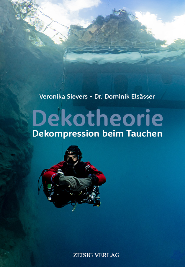
Let’s interrupt the regular program for a short commercial break: Veronika Sievers and Dominik Elsässer have turned their Punkfish online seminars into writing and finished a book on decompression theory:
So far only in German, it covers everything from the basics to the latest findings. It should be accessible to all divers and different from this blog does not assume you already know the basics. It’s a great read and I am not only saying that as I could contribute one or two of my nitpicks in the writing process. I like in particular that it contains a lot of references to the original research literature and pointers for further reading. It is available directly from the Nina Zschiesche’s (of Wetnotes fame) publishing house. Strong recommendation!
In the past, I have talked about the poor empirical data underlying the NOAA limits for preventing CNS oxygen toxicity. Of course, those are tricky, since having a seizure at depth has a high likelihood of resulting in fatal outcomes while there are good chances that the diver has no way to see it coming.
On the other hand, the limits have been quite restrictive: At a pO2 of 1.3 bar, you were supposed not to exceed 180 minutes in a single dive and 210 minutes in a 24 hour period. Sticking to such a limit (with 1.3 bar being a typical rebreather set-point) will make certain dives impossible as the decompression requirements exceed three hours. This had the consequence that many technical divers have been ignoring the limits coming from this “CNS clock”. Turns out, this has not led to many dead rebreather divers due to oxygen seizures at depth.
Turning this around, there is now more data to justify relaxing those limits while controlling the risk. In March 2025, at the American Academy of Underwater Sciences Annual Meeting, there was an expert workshop that resulted in new recommendations authored by Joseph Hoyt, F Gregory Murphy, Neal W Pollock, Dawn Kernagis, Nicholas Bird, Michael Menduno, John Bright, and Simon J Mitchell. They are still very conservative with their recommendations. For example, they only recommend new limits for pO2 of 1.3 bar although mentioning that it is highly likely that those times considered save would also be save at lower partial pressure. They make no statement about higher partial pressures like 1.4 bar or even 1.6 bar quoting insufficient controlled dive date in these ranges.
So, for 1.3 bar, they say, four hours of exposure during the “working part” of the dive plus an additional four hours during decompression at rest can be considered save.
They note that this is only about CNS toxicity as this has more potentially harmful consequences and pulmonary toxicity might have to be managed in addition. Furthermore they recommend considering additional safety measure like O2 breaks, breathing low density gases and using full face masks or habitats to mitigate consequences of a seizure.
PS: A few days ago, I had to learn that Michael Menduno, one of the authors of the paper mentioned above and editor of inDepth magazine has passed away. In the limited interactions I had with him he surprised me with is generous and welcoming attitude. Rest in peace!
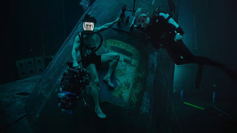
On Thursday, I took my daughter to the movies and we watched “Mission Impossible 8: Final Reckoning” which as my dear readers will be aware of involves an extensive under water chapter.
This leaves the theoretical diver with a number of questions regarding in particular the physics and diving shown. WARNING: Spoilers ahead!
Tom Cruise on the unter water set.
Why did they give him a dry suit and a prototype rebreather but forgot to give him fins? This makes him almost helpless in free water. He was lucky he basically fell on the submarine and did not miss it by a few meters which would have ended the mission immediately.
What is the depth at which he finds the submarine? I would think the Arctic Ocean is a few kilometres deep which makes it totally unsuitable for diving. On the other hand, in the final total it looks like not more than 20-30m which would make this whole decompression thing (and the prototype special rebreather) pretty much pointless.
Why did they put lights inside the full face mask to make sure he is constantly blinded? Why is the visibility so good and where does all the ambient light come from? (OK, a movie taking place for 15 minutes in complete darkness does not seem to be too promising)
The submarine supposedly exploded in 2012. Why is there still air inside? And once Agent Hawk opens the latch, why is the water only slowly tickling in? At any reasonable depth, I would expect the thing to be filled with water in the blink of an eye and crushing any human on the way.
To enter the torpedo tube, why does he have to take off his dry suit? And why does he use his knife rather than the zipper? Why can’t he take the rebreather with him? I am sure, the marine built it to fit into a torpedo tube.
The inflatable decompression chamber does not look like it could hold any significant pressure. And why is it built so big it can accommodate a romantic tete a tete? Why is he only one jump cut away from flying again on a plane?
I understand the kids today use generative AI for everything. So, it is just natural to use it to blend some diving gases as well. I already had my CGI script to compute how to top up your gases using Subsurface’s real gas approximation.
Now, I played around with some large language models and Claude.ai turned out to be able to rewrite this in JavaScript (which I don’t really speak but enough to put some finishing touches). As a bonus, there is no “Calculate” button but as in the Subsurface planner, you get instant results. You can find it here.
Everything in a stand alone html file that you can of course also install locally. You find in in the RealBlender Github Repository.
Here is an email I wrote to the Subsurface mailing list in response to the suggestion to offer the option to display gas use (SAC or RMV) in units of pressure drop per time even when you use only a single cylinder size:
There are two separate issues:
One is if you measure the gas consumption in units of
a) pressure drop per time
or
b) volume of gas at some reference pressure (typically surface pressure) consumed per time
the other is which term or abbreviation you use for a) or b).
Both discussions are very old already and Subsurface decided to call the measurement of b) „SAC“ or surface air consumption. It seems some other people call that RMV (respiratory minute volume) and maybe the latter ones are in a majority and Subsurface took a poor choice. I don’t know, maybe. In German, it is called AMV (Atemminutenvolumen which translates to breathing minute volume which is as stupid in German as it sounds in English but at least everybody uses it so there is no discussion). I don’t really care what you want to call it, maybe ABC is also an option or XYZ and I am open to changing the name in Subsurface if a large majority of English speakers say that one is the preferred term (but so far my impression is that there are people in both camps).
But the first issue is not up to discussion, the correct way do express it is b)! The only reason some people might think a) is a viable option is because in the water you have a gauge that measures pressure but you don’t measure amount of gas (as mols or volume at reference pressure) directly. So if you know how much your pressure gauge dropped in the last five minutes (assuming constant depth) you have a rough idea how many more minutes you can stay at the current depth and not running into gas problems. It gives you a rule of thumbs estimate but not more since future consumption depends on many other factors.
Once you are out of the water and write your log you can let your computer do the calculation to convert this into volume (amount of gas) units which is a much more meaningful way of expressing things. Others have mentioned that it makes no sense to compare pressure units if you you have different cylinder sizes. But even if you say you only have a single cylinder and will always use the same you should realise the conversion between pressure drop and amount of gas used is only simple in a world that knows only about ideal gases. Subsurface takes great proud in the fact it is aware this is only an approximation and takes into account the pressure dependent compressibility of breathing gases. And if you do that a pressure drop only translates to an amount of gas when you also know the starting pressure.
Let me show you in an example that this difference is actually relevant: I am diving in a world that uses metric units so my numbers come from common sizes an pressures in metric units but for your convenience I will translate those to imperial units (I guess you are using those because only in imperial units people have the idea that a) might be a meaningful thing):
Let’s do an air dive to 66ft (20m) for 22 minutes (i computed this in the planner) using D12 tanks (two 12 litre cylinder) with a total volume of 167cft.
If the pressure drops from 2900psi to 2320psi (200bar to 160bar) the SAC is 0.48cft/min (13.6 l/min).
If however the pressure drops from 1450psi to 870psi (100bar to 60bar), obviously the same difference in pressure, the SAC is 0.54cft/min (15.3 l/min).
So the difference in SAC (amount of gas used) is more than 10% if you start from a full cylinder or from a half empty cylinder and drop by the same amount of pressure. This difference in invisible if you measure it in pressure units but it is probably much higher than what you worry about when you look in trends of your gas consumption over time. (The reason is that at higher pressure air is significantly less compressible than at lower pressures).
You will not be able to seriously monitor your gas consumption over time if you use pressure/time units unless you always use the same cylinder and always start your dive with an identical starting pressure.
For this reason I am convinced that option a) is simply wrong (or for a less aggressive term: uninformed) and I will veto using it in Subsurface or even offering it as an option to the used (just as I would veto offering to turn off the real gas corrections even though we get many complaints about Subsurface getting gas calculations „wrong“).
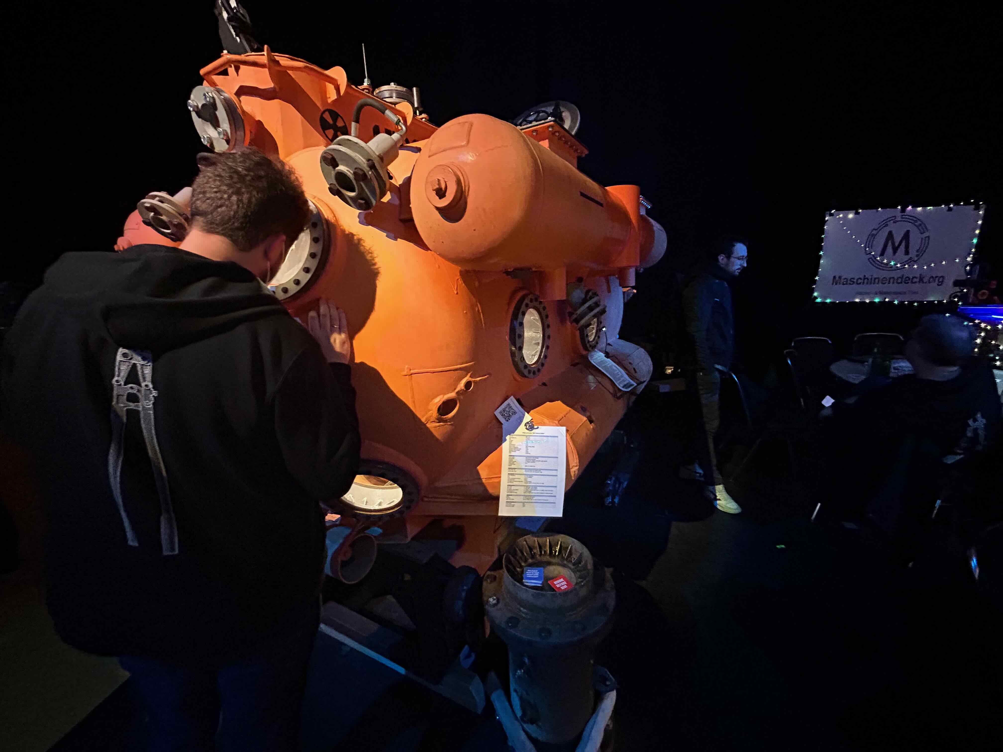
Not a lot of new content here recently. The last days, I attended 37c3, the annual hacker convention of the Chaos Computer Club which took place again in Hamburg . So, today, we will have some engineering content rather than the usual physics one.
You have to see the super entertaining talk by two guys who built their own submarine from scratch.
It has been very quiet here for a while. That is partly because there is a topic that I wanted to discuss here and since my take was going to be at least somewhat problematic, I felt for a while that I needed to do more reading to get the facts right. But now the time has come for me to talk about: Probabilistic decompression models.
The idea as such is very simple: Many models for decompression including the ones that I talk a lot about in this blog, Bühlmann, VPM-B and also DCIEM are “deterministic” models: They give you a plan and if you stick to it (or dive more conservatively) you should be fine but you must not violate the ceilings they predict at any given time. On the other hand, there are probabilistic models that aim to compute a probability of getting DCS for any possible profile and which you can then turn around and prescribe a maximal probability of DCS and then you optimise your profile (typically for the shortest ascent time) that gives you that prescribed probability of DCS.
That sounds like a great advantage: Don’t we all know that there is no black and white in decompression but there are large grey areas. Even when you stick to the ceilings of your deterministic model there is a chance that you get bent while on the other hand you do not immediately die when you stick your head above the ceiling, quite the opposite, there are chances that even with substantial violation of the decompression plan you will still be fine. That sounds pretty probabilistic to me.
Of course, things are more complicated. Also the deterministic models do not really aim at a black/white distinction. Rather, they are also intended to be probabilistic but with a fixed prescribed probability built in. For recreational diving (here as usually including technical diving but not commercial diving), the accepted rate of DCS is usually assumed to be one hit in a few thousand dives. That seems to be the sweet spot between not too often having to call the helicopter (and most recreational divers never experiencing a DCS hit) and being overly conservative (too short NDL times, too long decompression stops). So, the only difference is that for the probabilistic models, this probability is an adjustable parameter.
You can turn this around: Why would you be interested in dive profiles that have vastly different probabilities of DCS that this conventional one in a few thousand? After all, even for one possible value of p(DCS) it is very hard to collect enough empirical data to pin down the parameters of a decompression model. Why on earth would you want to do that also for probabilities that you do not intend to encounter in your actual diving? Why would I be interested in computing an ascent plan that will bend me one dive in twenty for example? Or in only one dive in a million? That sounds to be overly complicated for useless information.
The answer is exactly in your restricted ability to conduct millions of supervised test dives: Let us assume you have a probabilistic model with a number of parameters that still need to be determined empirically. But you have a priori knowledge that the general form of your model is correct (we will come back to this assumption below), you can do your test dives with depths, bottom times and ascents that your model gives you DCS probabilities in in the range of 5-50% say, depending on the parameters. Much more aggressive than you intend to dive in the end. But such test dives will give you a lot of DCS cases and you do not need too many dives to determine if the true probability is 5%, 20% or 50% and adjust the model parameters accordingly. You gain already a lot of information with just 10-20 dives while for dives with the 1/10000 rate of DCS you need many more dives to have enough DCS cases to establish the true probability.
Once you have established the parameters of your model with these high risk dives where you have to use your chamber a lot to treat your guinea pig divers after bending them you can then use your model for dives that have a much healthier conservatism where your model gives you for example p(DCS)=1/10000.
An example of doing your study in a regime where you expect to bend many contestants is the famous NEDU deep stop study where the divers were in quite cold water with insufficient thermal protection and in which they had to work out on ergometers while in the water all to drive up the expected number DCS cases (there not necessarily with a probabilistic model in the background but just the intend to see a difference in deeper vs shallower decompression schedules where of course 0 DCS cases for both ascents wouldn’t be very informative).
But as so often, there is no such thing as free lunch: You are extrapolating data! You make experiments in a high risk regime of your data and then hope that the same model with the same parameters also in a low risk regime. You are extrapolating your data over several orders of magnitude of probability. This can only work if you can be sure your model is correct in its form and the only thing to determine empirically are the few parameters. But in the real world, in particular in decompression science, such a priori knowledge is not at hand.
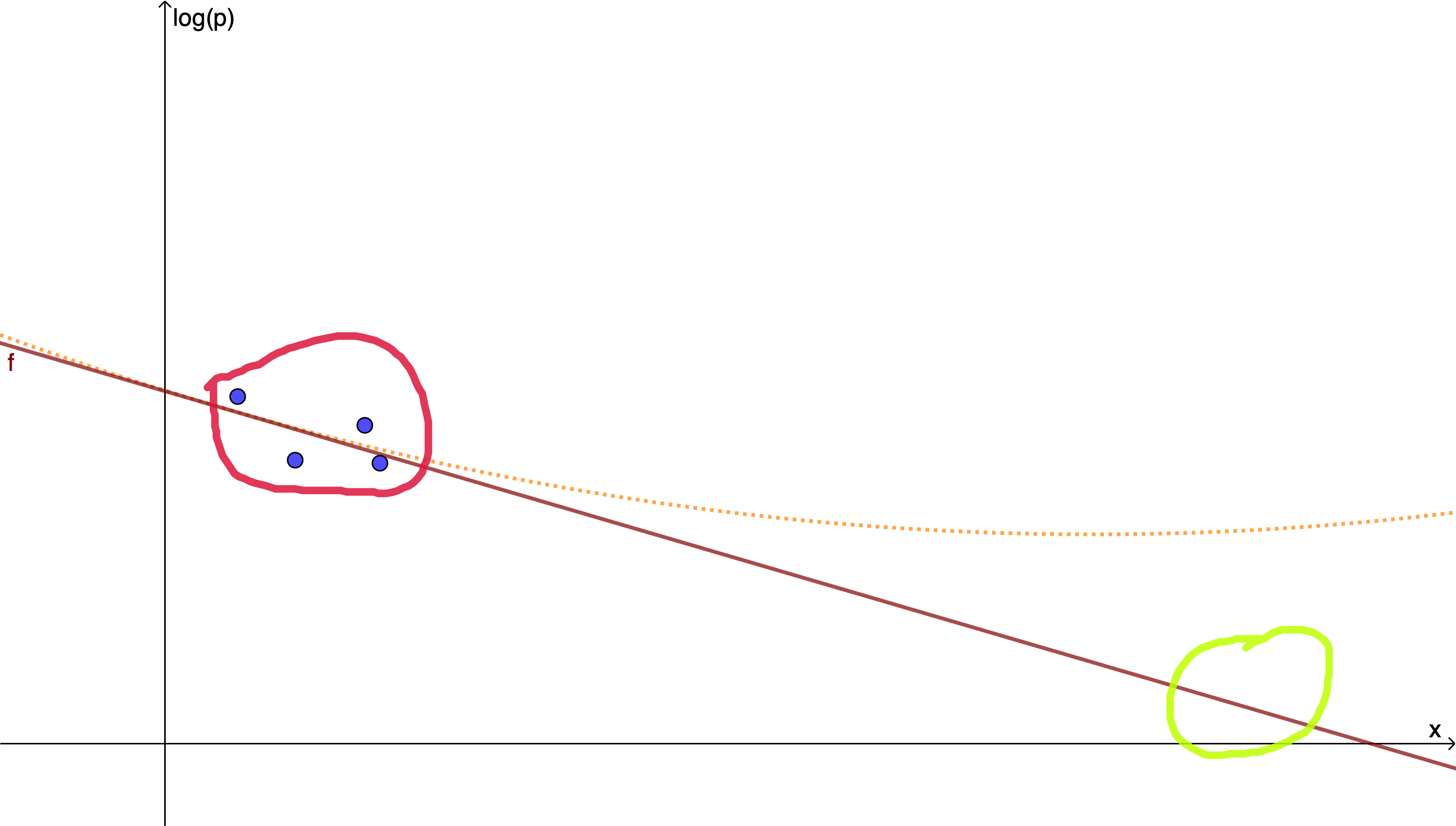
Let me illustrate this in a simplified example: Let’s assume, there is only one parameter x and your model is that the logarithm of p(DCS) is a straight line (an affine function) of x
\(\log(p_{DCS}) = m x +b\)
Then, in your experiments you do a number of test dives at various values of x, find the corresponding rates of DCS and finally fit the slope m and the intercept b by linear regression.
The red area is the high risk regime where the model is tested, the green are where it is supposed to be applied. If the reality is not a straight line (solid) but there is small quadratic component (dotted) the difference in the green are can be significant while the fit to the experiments in the red area is still good.
If however the a priori assumption of the model that a straight line does the job is not justified because there is also a small quadratic contribution, say, you can fit your parameters as closely as you want but still get very far off in the extrapolation to where you intend to use your model.
This is of course only an example and for more complicated models you will use a maximum likelihood method to find optimal values of your model parameters given the outcomes of various test dives. But what this will never be able to do is to verify the form of your model assumptions. You are always only optimising the model parameters but never the model itself. For that you need independent knowledge and let’s hope you have that.
VVAL18
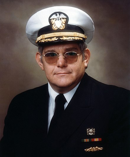
To be specific, let us look at one probabilistic algorithm more concretely: VVAL18 which was developed by Edward Deforest Thalmann for the US Navy based on a database of a few thousand navy dives. For military divers, the accepted risk of DCS is much higher, if 2% of the dives result in symptoms that need to be treated that is still considered fine given that decompression chambers are typically available at the dive spot. This model is also known as the Thalmann algorithm and is described for example in short in this technical report. (Similar things could for example be said about the SAUL decompression model which is similar in spirit and also inspired by the navi data)
E.D. Thalmann (Wikipedia)
This model also uses compartments with half times but leaves open the possibility that the partial pressures do not follow the usual diffusive dynamics with the rate of change proportional to the pressure difference to the surroundings but for off-gassing also allow for the possibility of a constant rate (which leads to linear rather than exponential time dependence).
For each compartment i, there is a fixed threshold pressure pth that as an excess pressure is considered harmless and above that a relative excess pressure is calculated
\(e_i = \frac{p_i-p_{amb}-p_{thi}}{p_{amb}}\)
To compute the risk, for each second of the dive and each compartment, risk of not getting bent in the second is assumed to be
\(e^{-a_ie_i}\qquad (*)\)
for some constants ai. Finally, all these individual risks are considered to be independent, so the “survival probability”, the probability of not developing DCS is assumed to be simply the product of all the individual probabilities for compartments and seconds (since they are in the exponent, you can there integrate the ei over time and sum over tissues).
These constitute the a priori assumptions of the model that I was talking about: The exponential dependence of risk on relative overpressure (*) and the statistical independence of tissues and instances of time. According to these assumptions, your risk of DCS increases exponentially in time when you do longer decompression (assuming the excess pressure is kept constant) for deeper dives or longer bottom times (this is clearly at odds with the assumptions of for example the Bühlmann model that allows you to have arbitrary long decompression obligations as long as you do not violate a ceiling) and you are allowed to have arbitrary large excess pressures if you keep the duration of the excess short enough (tell that to your soda bottle).
With these assumptions, for which I could not find any justification in the literature for, except “we came up with them”, lack of imagination, then the parameters of the model are optimised using maximum likelihood. In the Thalmann case, there three tissues and the parameters to be fitted are the half-times, the thresholds pth and the constants ai.
The three half-times Thalmann ends up with are roughly one minute, one hour and ten hours (with large uncertainties), the thresholds are essentially 0, and the ai are in the 1/50000 range (you can find the values in an appendix of the report cited above, note that time units of minutes are used rather than the hypothetical second I used here).
I have serious doubts about the intrinsic assumptions of (*) and the statistical independence of time segments. But for Navi use where you accept DCS risks of a few percent those may be ok since any model with sufficiently many fitted parameters will reproduce dives with similar parameters. But failed assumptions will bite you when you extrapolate your model out from the high risk regime to recreational diving as failed model assumptions tend to blow up under extrapolation.
I want to mention that I am grateful to the LMU Statistics Lab that I could discuss with them some of the issues mentioned. Of course all mistakes here are my own.
This post is a copy from an answer in the Subsurface support forum but I post it here as well as this point comes up over and over. It is about the setting of some dive computer where you can set the density of water or whether you are diving in sea or fresh water. There is a similar setting in Subsurface, but the default setting in the preferences is to hide it. For a good reason.
Let me mention once more why this option is turned off by default: There is a good chance that by fiddling with the density you make changes whose effects are not what you intend: The density is the relevant constant that controls the conversion between depth and ambient pressure. That you probably intend. But what is easy to forget: Your dive computer displays depth and reports it in the log that is transferred to Subsurface. But it does not really measure depth, rather it measures ambient pressure and it uses the density to convert that to depth.
It does this conversion because we humans are used to think in terms of depth which is much like a length and we have an idea how much 10m is, much more so than 2bar.
For most things diving, however, depth does not matter at all, ambient pressure does. This includes gas consumption (as your regulator regulates according to ambient pressure, not to depth) and all deco calculations (because also there partial pressures in their relation to ambient pressure dictate what is happening in your body). Depth only matters when you think about breaking a new world record or worry if the mast of the wreck sticks out of the water or if you buoyo line is long enough. For gas usage estimates and deco calculations, it would be much more honest if your computer displayed ambient pressure in bar rather than depth in m. Only that for the average Joe that would be hard to digest and we have to live with the fact that this conversion is done back and forth by the computer and by Subsurface all the time.
But what really makes zero sense is to use different values of density when translating back and forth. Also your dive computer does not measure the density, this is a setting that you have to make manually. Yes, you could change that setting on your dive computer every time you switch between sea and fresh water to get a more accurate depth display (which as I explained above most likely does not matter at all). But my guess would be you forget to change that setting for at least half of your dives. So my very strong recommendation would be to set it on your dive computer once and for all to any value (maybe according to where you do most of your diving) and set Subsurface accordingly and never ever change it again. The result can be that some of your depth readings are slightly off but at least your gas and deco calculations will be consistent.
As mentioned before, gases in diving cylinders are not only not sufficiently well approximated by the real gas equation but also the van der Waals equation, despite its prominence in thermodynamics teaching, is not doing much better.
Subsurface does better than this using a polynomial fit to table data for the compressibility of the three relevant gases. In a discussion at ScubaBoard, the question came up how to use this in gas blending. After an initial version using Mathematica, I sat down and implemented it as a perl script and hooked it up to this web page for everybody’s use and enjoyment. Here it is:
source code is on GitHub. Right now, it does only nitrox. But it computes instructions to up up partly filled cylinders with any pre-existing nitrox mix.
Let me know if you think extending it to trimix would be useful for actual use. I am not sure what the best user interface would be in that case: For nitrox, specifying the initial and target mix and pressure and two top up mixes, the blending problem generally has a solution. But with three gas components to get right, it is in general impossible with only two top up mixes. So you either have to use three (linearly independent) top up mixes or let one thing unspecified. That could be either the oxygen or helium fraction of the final mix or you have to leave open one of the gas fractions of the top up gases.
So what do you do in practice, which component do you leave unspecified?
Update: I updated the script so it can now also handle blending trimix (starting from a partially filled cylinder, you can specify three top up gases it will now calculated the intermediate pressures you have to fill up to). To blend nitrox, specify the target mix as containing no helium and leave one of the top up mixes empty.
Update: I discovered an error in the calculation (I calculated the mix according to pressures rather than volumes at 1 bar) that should be fixed now (April 10, 2022)
When the Subsurface mailing list recently received the request if the planner could implement the DCIEM model as well my first reaction what “Whut?” has I had not heard of it before.
Turns out, DCIEM stands for “Defense and Civil Institute of Environmental Medicine” which was a research institution of the Canadian military and is now part of DRDC Toronto according to Wikipedia. The request to Subsurface was apparently prompted by the fact that Shearwater announced to implement the model into their dive computer for commercial divers. The “for commercial divers” sounds to me like this is more to tick some boxes in the health and safety requirements for these people rather than something that the diving world at large should adopt. But still, it might be interesting to see what this model actually does.
Some googling suggests that this model is mainly consumed not in terms of an algorithm in planning software or dive computers but in the for of tables. A 1992 version can for example be found here.
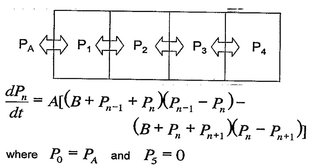
But Google also finds a review paper by Nishi and Tikuisis that explains that the DCIEM model is a non-linear model developed by Kidd and Stubbs. It shows as four compartment discretisation of a slab of tissue together with a ODE for time evolution:
Kidd-Stubbs model according to Nishi and Tikituisis
As written, I cannot make much sense of it but things clear up when the expression is expanded:
\(\dot p = ab \Delta p +a\Delta p^2\)
Here, p is the vector of tissue pressures and Δ is the discrete Laplacian that for a sequence (s) is
\( \Delta s_{n} = s_{n-1} -2 s_n + s_{n+1}.\)
If there were only the first term on the RHS, that would simply be a diffusion equation that I would also have written if somebody had asked me to write down a model for a slab of tissue. I have no clue where the second, non-linear term comes from but clearly it can safely be ignored as long as p<<b. There is also a paper by Nishi and Kuehn that gives a FORTRAN implementation of the model (doesn’t this sound familiar…). In the source code, I find a value of b=274.5 which is supposedly in units of psi which translates to 19bar, so the non-linear term should will not be relevant for anyone with a depth limit short of 200m. In the review paper it is stated that the constants of the model were fitted to bubble measurements after trial dives but one could wonder how this is would be possible unless compartment pressures at least came near to 20bar…
The paper with the FORTRAN program also explains that the relation between tissue pressure and ambient pressure is pretty much a standard \(p_{amb}\ge c_1 p_{tissue} + c_2.\)
More interesting is that the discretised slab is an example of the interacting tissue models I talked about in the post about those being equivalent to independent tissues. For four tissues, the discretised Laplacian (there is of course also a closed form) has eigen values \(\frac{-3\pm \sqrt 5}{2}, \frac{-5\pm\sqrt 5}{2}\) which numerically range between -3.6 and -0.38.
So, the four independent tissues after diagonalization cover one decade of half-times all proportional to 1/ab.
So, taking everything into account, the DCIEM model is (equivalent to) a Bühlmann type model with four tissues coving a somewhat small range of half-times. So I would expect with an appropriate choice of constants, one can produce somewhat reasonable deco schedules at least for air dives (we have not discussed different gases) with not too long runtimes. But a full blown Bühlmann (possibly with gradient factors) is much more expressive.
Hinweispflicht zu Cookies
Webseitenbetreiber müssen, um Ihre Webseiten DSGVO konform zu publizieren, ihre Besucher auf die Verwendung von Cookies hinweisen und darüber informieren, dass bei weiterem Besuch der Webseite von der Einwilligung des Nutzers
in die Verwendung von Cookies ausgegangen wird.
Der eingeblendete Hinweis Banner dient dieser Informationspflicht.
Sie können das Setzen von Cookies in Ihren Browser Einstellungen allgemein oder für bestimmte Webseiten verhindern.
Eine Anleitung zum Blockieren von Cookies finden Sie
hier.