Uncategorized – Page 4 – The Theoretical Diver

VPM-B for real dives (or not)

The VPM-B model (of which I have described my understanding in previous posts) has a “derivation” in terms of bubble physics which I, as readers should have noticed, have some trouble to follow through completely as it is, to say the least, ad hoc and sketchy in places. I bet, only based on this derivation in prose plus formulas, nobody would be able to write a program to compute a VPM-B deco plan.

But we are lucky: There is a reference implementation in terms of a FORTRAN program. So, even though the VPM-B code in Subsurface is a complete rewrite (and solves many things algorithmically differently than the original code), we did a lot of testing to make sure that the plans we produce are identical to the plans computed using the FORTRAN program, even in places where we thought it makes little sense (like starting the ascent to the next stop when the ceiling depth equals the depth of the next stop rather than starting a bit earlier and making sure never to violate the ceiling during the ascent to the next stop (which is different since the ceiling goes up during the time it takes to get to the next stop). The latter is, at least to me, better motivated physically (“simply never violate the ceiling”) than basing the stop time on what happens at a different depth (namely the next stop depth) and we use the latter when computing Bühlmann schedules. But for VPM-B, we thought, given that we do not really understand the physics, we should not modify the model based on physics.

I have talked in the past about the Bühlmann model not being well defined to make all implementations come up with identical plans. In a sense, we are in a better situation with VPM-B, since there is the FORTRAN program which (at least for us) defines the model. But the problem is: This definition works only for the situation that you can compute with the FORTRAN program: You specify the bottom part of the dive and then let the program work out the ascent. Strictly speaking there is no definition for real dives: Dives where the distinction between bottom part and deco is blurred. But this is exactly what you have if you were to implement it in a dive computer or, as for Subsurface: Implement it in a dive log to show a ceiling for a logged dive (after all, Subsurface is mainly a divelog). For real dives, you cannot tell the exact point where bottom time ends and deco begins.

Unfortunately, the model depends on this: As explained in the VPM-B derivation post, one parameter that goes into the computation is the total deco time $t_D$ (clearly that ends when you reach the surface, but where does it start?) but there are other parameters that you are supposed to evaluate at the beginning of the ascent like $p_{1st ceiling}$ and the initial gradient for the Boyle compensation. All this depends on the time you call the end of bottom time and thus the computed ceilings also depend on that.

For Subsurface, we decided to take the point of time with the deepest ceiling (which, strictly speaking, is a circular definition but in practice is irrelevant) as the end of bottom time and base the ceiling computation in logbook mode on that. But that, to some degree, is arbitrary. And even for dives that we planned using VPM-B (and thus agree with the schedules computed by the FORTRAN program), applying this logic yields a slightly different ceiling. So it can appear that a VPM-B planned dive violates the VPM-B ceiling. But this is only due to the fact that the model is not really defined outside the planning situation.

Or put differently: You need to make arbitrary assumptions (not based on the depth profile and the gas you are breathing) to come up with a VPM-B ceiling. Which, at least for me, doesn’t strengthen my believe into this model.

PS: I am planning to be at the Boot dive show in Düsseldorf on Friday January 26th. If you happen to be there as well, please let me know and we can shake hands!

DIY on the fly

With the new version of Subsurface out today, I would like to point to a feature that was already there in 4.7.4, but which just got more usable: Computing deco variations in the planner.

This is motivated by the discussions about Ratio Deco and Deco On The Fly, for a discussion see this post by Rick. These approaches to computing deco are not really attempting to model anything that is supposed to go on in the diver’s body but simply to take a very pragmatic approach and interpolate deco schedules from known ones. If you like, they are (or attempt to be) mnemonics to learn deco plans by heart. The idea is simply that you memorise a reference plan and also how you have to modify deco if you modify the bottom part of your dive.

With Subsurface, you can now do exactly this: You can take any dive that you planned in the planner as reference dive and it will tell you how your total deco time depends on the bottom part. Take for example this trimix dive to 60m with 30min bottom time:

The runtime table says

The important line is the second:

Runtime: 118min, Stop times: + 3:05 /m + 3:59 /min

This tells you how to adjust the total deco time when changing the bottom time (the segment at 30m): For each meter that you go deeper, you have to add about three minutes (for example if you went to 63m for half an hour, you would have to add about 9 minutes or if you only went to 58m you could shorten your deco by 6 minutes). Similarly, if you change the bottom time you have to pay every extra minute on the bottom by about four minutes in deco.

It does not tell you how to distribute this time over the different stops but a good rule of thumb would be to do it roughly proportional to the time you already spend at the stops. So for example, of the about 90min of total deco time you spend roughly half at 6m, you would also add half of the extra time at this last stop.

These numbers are supposed to be something like the partial derivative of the total deco time with respect to depth and duration of the bottom time element (actually: the last manually entered part of the dive). You are supposed to multiply these derivative with the actual variation of the bottom segment that you do.

How do we compute these numbers? When this calculation is enabled, Subsurface actually computes five extra plans: It first computes the original plan, but now with second resolution of the stops instead of minute resolution. Then it shortens the bottom segment by one minute and computes the plan (again to seconds) and then computes a plan for a bottom time extended by one minute. Then it computes to more plans for one meter shallower and one meter deeper.

This give us two time differences both for depth and duration variations. What is displayed is the average of those. But a bit of experimentation shows that the difference is typically only a few seconds (and what are seconds for 90min deco?). This is also a measure how good this linear approximation is (as this the quadratic correction): It gives me confidence to say this approximation isn’t too bad for a few minutes or a few meters.

So having these two numbers also on the runtime table should give the diver much more confidence in how to react to unforeseen changes of plan (both shallower and deeper and shorter and longer). But of course, always remember: Plan the dive, dive the wreck, wreck the plan!

CCR Schreiner Equation

Since there was a question on Scuba Board about how to compute the tissue pressures when diving a CCR (i.e mainlining constant partial pressure of oxygen) when changing depth at a constant rate. When putting this on a computer I would say doing it for small time steps and pretending to be at constant depth for that short amount of time doesn’t do much wrong and you will end up doing this anyway (at least that’s what we do in Subsurface). But for the fun of it, let’s work out the analytic solution.

Let’s start by figuring out the inert gas ambient pressure at a given depth. We call $p_d$ the diluent partial pressure, $p_{O2}$ the partial pressure supplied from the oxygen cylinder (note that this is not the oxygen partial pressure since there is going to be some oxygen in the diluent as well), $d$ is the depth, $f_{O2}$ is the fraction of oxygen in the diluent while $f_i$ is the fraction of the inert gas we are computing in the diluent.

There are two obvious equations: The ambient pressure is equal to the diluent pressure plus the oxygen pressure in the loop:

$$ p_d + p_{O2} = p_a = p_{surf} + dg\rho$$

Here, $p_{surf}$ is the surface pressure, and $\rho$ is the density of water and thus $g\rho$ the conversion factor between depth and pressure. The second equation says that the total partial pressure of oxygen (from diluent and oxygen cylinder combined) has to equal the set point pressure $p_s$:

$$f_{O2} p_d + p_{O2} = p_s.$$

We can subtract both equations to eliminate $p_{O2}$ and find

$$ p_d = \frac{p_{surf} + g\rho d -p_s}{1-f_{O2}}.$$

This goes into the usual diffusion equation for the inert gas loading in the tissue $p_t$ that we are ultimately interested in:

$$\dot p_t = -\gamma( p_t -f_i p_d).$$

$\gamma$ is the usual diffusion constant that is related to the inverse of the tissue half-time by a factor of $\ln(2)$. Finally, we want the depth to change linearly in time, so $d=d_0+vt$ where my sign convention is that $v$ is the descend velocity, make it negative for ascends.

So we have to solve a linear inhomogeneous ODE with constant coefficients which we could tackle by “varying the constants”, but of course we are lazy and let Mathematica do the job. After a bit of massaging, we find

$$p_t = \frac{f_i}{1-f_{O2}} \left( e^{-\gamma t} -1\right) \left( p_s + \frac{vg\rho}\gamma\right) + e^{-\gamma t}\left( p_0 – \frac{f_i}{1-f_{O2}} (p_{surf} + d_0g\rho)\right) + \frac{f_i}{1-f_{O2}}(p_{surf} + dg\rho)$$

where $p_0$ is the initial tissue loading. So, here you go this is the CCR Schreiner equation. Or, if you want to follow the tradition to attaching names to simple solutions of ODEs, I allow you to call it the Helling equation.

Update: If you are worried that a constant water vapour pressure has not been taken into account, you can bring it in by replacing the set point by the actual set point plus the water vapour pressure in all equations above.

We moved

Finally, The Theoretical Diver is on its own domain thetheoreticaldiver.org . I had intended this move for a long time but it became necessary as the ancient WordPress instance had uninvited visitors (don’t get me started on why it was impossible to update that beyond mentioning that the OS version of the host of that blog required me to run a very old Debian release which came with an old PHP version which only allowed a WordPress version from about the time when my grandma went to elementary school).

So here we are now. And since WordPress does not really like to be moved to a new domain (yes, they store absolute paths in their database, no clue why) and backing up the old was also difficult given how old the WP version was (which excluded most plug-ins) I moved all posts essentially bu cut&paste. I tried to update all the links as well. But please let me know if you find something outdated.

What I couldn’t move are the comments. Which is a pity.

So, once more, welcome to the new site! I hope you feel at home.

N2 vs. He, what’s the difference?

Recently, a blog post on the Shearwater blog was pointed out to me (thanks Jan) that reports on a paper by David Doolette etal and the Navy Experimental Diving Unit comparing the same 200ft dive with 40min bottom time both on a CCR rebreather once with trimix 12/44 as diluent and once with 12/88 (i.e. heliox) as diluent. Divers followed a deco plan computed for trimix and the traditional wisdom would have been that a fraction of the heliox divers would get bent thanks to an increased amount of helium in their body. But the study found that this is not the case and only some of the test divers breathing trimix were getting bent.

The NEDU trimix dive replaced with Subsurface.

Here is the dive replanned in Subsurface. One would need gradient factors 110/36 (low/high, note the order!) to come up with this plan, but ok, fine. Notice the unusual pattern on the heat-map.

The upshot apparently is that traditionally one was overestimating the penalty for using lots of helium in short bounce dives (from the perspective of the navy). Helium atoms being much smaller than nitrogen molecules are believed to diffuse much faster into the body and thus prompting deeper stops.

Obviously, this cannot be the whole argument since faster diffusion would also lead to faster desaturation, so here is a post to look a bit deeper into the differences between nitrogen, helium and trimix from the deco perspective. Since this is easiest to understand in its consequences, let us discuss these matters from the perspective of the good old Bühlmann model.

I think it is indeed not controversial that smaller particles diffuse faster but that alone should make zero difference! This might sound surprising but let’s look at Bühlmann’s list of half-times (these are essentially inverses of the diffusion constants). Those are for nitrogen (in minutes):

const double buehlmann_N2_t_halflife[] = { 5.0, 8.0, 12.5, 18.5, 27.0, 38.3, 54.3, 77.0, 109.0, 146.0, 187.0, 239.0, 305.0, 390.0, 498.0, 635.0 };

const double buehlmann_He_t_halflife[] = { 1.88, 3.02, 4.72, 6.99, 10.21, 14.48, 20.53, 29.11, 41.20, 55.19, 70.69, 90.34, 115.29, 147.42, 188.24, 240.03 };

Obviously, there is a difference. But how did he measure those? The answer is: He didn’t. You can come up with those (starting from N2) only by theoretical reasoning. You assume that the relevant physics is diffusion. And that has only one parameter, the diffusion constant or half-time. And that you don’t know a priori. But you can imagine that you only need to look at processes at time scales compared to those encountered during a dive. And there, pressure changes at the order of a few minutes and the total dive length which is a few hours. So anything in between will be relevant. And this is what gives you those numbers! They vary from five minutes to 10.5 hours. Ideally you want to cover the whole range of in-between numbers but of course you can do this only for a finite number of values (here taken to be 16) which you then evenly spread in the interval. Where evenly means that consecutive ones differ by the same percentage (rather than absolute value), i.e. they form a geometric progression. And, guess what, they do.

Obviously, there is a bit of arbitrariness in this procedure, in particular in picking the smallest and the largest value and in the number of intermediate steps. But as long as the slowest or fastest compartment are not the leading compartment for a larger part of the deco and the gaps between adjacent tissue half-times are not too big, those choices should not really matter.

But this means that what seems to be the biggest difference between nitrogen and helium, the difference in half-times is really no difference at all! It only means, we parametrize the range of possible diffusion constants differently. Yes, compartment number four has a different half-time for N2 (18.5min) than for He (7min) but there are compartments six and seven (half-times 14.48min and 20.53min) which would cover the same time range. (Note that thanks to the diffusion equation, the tissue loading after time is the Laplace transform of the ambient pressure and according to the structural similarity between Laplace and Fourier transform, the half-time plays the role of a frequency, so a tissue gets particularly excited if the ambient pressure changes at the same time scale which is like exciting on oscillator with its resonant frequency).

Keep in mind that “the tissue” does not really correspond to a certain part of the human body like muscles being modeled by compartment x and bones by compartment y (even though some layman’s explanations make you believe that), rather the range of tissues models the range of diffusion constants and our ignorance about the time constants that might play a role in a complex system like that of a diver during the dive.

So, if you did one dive in which the breathing mix contained a given fraction of nitrogen, then the tissue loading of compartment four would be the same as if the same profile would be dived with breathing a mix that contains that fraction now in helium and then in compartment six or seven (ignoring the fact that before the dive, at the surface you were breathing air and not heliox 79).

So much for tissue loadings (where the difference between N2 and He is only in a shift in compartment number). But what about M-values (parametrized by a- and b-coefficients in Bühlmann’s model)? Those are different for He and N2.

Yes, they are. When indexed by compartment numbers. But we just saw, those don’t mean much, we should rather look at them as a function of half-time. And then the difference is much smaller as can be seen by these diagrams:

Orange is helium, blue is nitrogen. There seems to be a systematic difference for slow tissues for a and for fast tissues for b but this goes essentially away once one plots the tolerated ambient pressure (the “M-value”) as a function of tissue loadin according to the linear equation

$p_{tol}=(p_{i} – a) \times b$

M-values for He and N2 as a function of tissue pressure and half-time

This plot shows $p_{tol}$ as a function of (the log) of the half-time and the tissue loading and one sees there is hardly any difference between the orange and the blue surface (here is a version that you can rotate to look at it from all sides without coordinate frame though, thanks Mathematica). I computed all these plots in a Mathematica notebook that you can download here.

Again, the upshot is that once you align the tissue half-times, the difference between the two inert gases is quite small. So, why is there a “penalty” for using more helium in your mix (while there above mentioned study finds evidence for not so much difference)? Where does it come into the model?

The answer is that when actually diving trimix, that is having both N2 and He in your mix, one has to combine the effects of the two. In the Bühlmann model, you are supposed to add the partial tissue pressures and use the weighted average (weighted by the fractions of the two inert gases) of the M-values. And here it is, where you combine them using tissue number (and not as I did above) by half-time. The justification would be that due to the different diffusion rates this is what happens in a single tissue in the body (with the above mentioned caveat that these tissues are theoretical constructs of an interpolation and not necessarily reflect real physiological tissues).

The effect is that now some nitrogen load is compared to an M-value which partly comes from He which gives you a much stricter M-value (as the He-M-values are smaller when you compare them with aligned compartment number rather than half-time). This is where the penalty comes from.

To me it sounds as if it is this combining of the gases is actually the part of the Bühlmann model with the weakest justification from a physics point of view. And my interpretation of the NEDU study is that it supports doubts that this is the right thing to do.

It seems, further studies about this part, where one simply takes two gas compartments which happen to have the same compartment number (which is only a coordinate in diffusion constant space after all) and throws them together for the two different gases, are needed. At least, this is where I would put my money that this is an area where the models could be improved (or at least better empirically justified).

Update: In a previous version I had claimed that David Doolette had invented the heat-map display of decompression. It was pointed out to me that this was in fact user “UWSojourner” on several fora.

When real gas corrections matter

We have all learned that most of the time the ideal gas law (maybe in its isothermal version known as Boyle-Mariotte law) is sufficiently accurate to calculate the amount of gas in cylinders. At least as long as we restrict to pressures not exceeding about 200bar (and of course we all know it’s a beginner’s mistake to assume 300 bar cylinders give you a 50% advantage in gas carried with respect to 200 bar cylinders even forgetting the problems of actually getting those filled to nominal pressure or attempting to mix in at those pressures).

But let’s look at this a bit more quantitatively: You can parametrize the error of the ideal gas law by a “compressibility factor” Z so that it becomes

$pV = ZnRT$

and then tabulate Z as for example done here. In the table for a realistic temperature of 300K you read off 1.0326 at 200 bar while only 1.0074 at 150 bar. So, at 200 bar, you overestimate the amount of gas in your cylinder by 3% or put differently, the amount of gas is that of an ideal gas but only at (1-3%) 200 bar = 194 bar while the amount calculated at 150bar is almost correct.

What is 3% amongst friends I hear you complain, that is likely less than the accuracy of your pressure gauge. That is of course correct but lets see how this relative error multiplies as soon as you take differences: Let’s say you want to compute your surface air consumption (SAC) for a dive in which you breath your cylinder down from 200 bar to 150 bar. Wrongly assuming the ideal gas law to hold lets you compute the amount of gas to be 50 bar times the volume of your cylinders. But as we saw, due to the compressibility factor, we should rather use 194 bar – 150 bar which is only 44 bar. Compared to the 50 bar of the ideal gas, we now have a 12% error, something that I would already consider significant. In particular when I use this value to extrapolate the gas use to other dives.

We see that suddenly the relative error multiplied by a factor of four and for the momentary gas use one needs to look at $\partial Z/\partial p$ as well.

The upshot is that even for 200 bar one should better use a real gas replacement to the ideal gas law. Anybody who had been in an undergraduate physics class would now probably go to van der Waal equation but as it turns out for typical diving gases in the commonly used pressure ranges that gets 1-Z rather poorly. So for Subsurface we had to use a more ad hoc approximation. But that is the topic of a future post.

What is this?

Welcome to my new theoretical scuba diving blog!

What is “theoretical diving” you will probably ask. Let me explain. By day, I work as a physicist at Ludwig-Maximilians-Universität München, as a theoretical physicist more specifically. But I also like a lot to go scuba diving. Unfortunately, I do not have as much time anymore to go diving as I used to have (for a variety of reasons). So instead, I like at least to think about diving. And I think about it as a theoretical physicist. In this blog, I would like to share what I came up with thinking about scuba diving.

Besides this blog, another theoretical diving activity of mine is contributing to Subsurface, the open source dive logging software started by Linus Torvalds and Dirk Hohndel. In particular, there I try to contribute to decompression calculations and the dive planner. In the course of working on that program, I also keep learning things (besides how to work in an open source project) that I would like to share here.

The plan to start this blog (besides my regular which means mainly physics blog) has been there for almost two years. So let’s see at which rate I manage to write posts. I hope I can also find some other contributors.

So, here we go…

VPM-B: How it works (the no non-sense version)

One of the features that Subsurface users kept asking for were other deco models besides Bühlmann (including gradient factors). In particular, they wanted to see a bubble model implemented. I was reluctant to do so for some time since I believed (like many other divers) that you can produce fine decompression profiles that look like they are coming from a bubble model by using gradient factors, in particular by using settings like ${GF}_{low}=20-30$. But more important: I did not understand how they worked.

And this is not because I cannot understand how you can derive this or that formula from physical laws (I do that for a living), but because the text that are supposed to describe these models appeared to me to be confused. There were huge gaps in my understanding of the original texts, like this or this, those seemed to me like spending a lot of space on absolutely trivial calculations (like integrating an exponential function) while on the other hand not clearly saying what the actual strategy is and what all those symbols meant. Plus some of the derivations seems to use some slightly unorthodox algebra… There are other texts by other authors that are clearly derived from these originals but I keep having the impression that those secondary authors did not understand the difficult parts either, since many of them are just paraphrasing the originals.

For RGBM there is no hope of understanding it since its inner workings are a trade secret. But the situation of VPM-B is actually better: There is a very concise definition of the model. But it comes in the form of a FORTRAN program by Eric Baker. It is about 75 pages when printed out on paper and it is FORTRAN, so again, the core of the algorithm does not directly present itself to the reader.

Somebody had run this FORTRAN program through f2c but of course the resulting C code is not any more readable. But at least, that allowed be to single step through it with a debugger (rather ran running my finger through 75 pages of spaghetti code). Since then, there are a few more implementation, Since then there are a few more implementations including the C version by Bryan Waite which is at least idiomatic C. But still it follows pretty much in a 1:1 fashion the original FORTRAN code including the separation into sub routines and variable names.

But last summer, there was the opportunity to have a Slagvi, a Google Summer of Code student work on this and do a VPM-B implementation from scratch. I was his mentor and this here is what I learned. Slagvi’s task was not just to link the existing code to Subsurface but really do a reimplementation so that in the process we could understand what is actually going on (and what part of the “explanation” is just a smoke screen).

You can find the result in the subsurface source code, in particular in the two files deco.c and planner.c.

This post here is a start of a series of (to be written) posts that aim at a fresh presentation of how VPM-B works. The next looks at the actual algorithm.

VPM-B: How to compute your deco

This is the first technical post about the inner workings of the VPM-B deco model. Here I will just present the algorithm (including the relevant formulas, some of them maybe in an unusual form) while the physical motivation or derivation will be the subject of a future post.

I try not to parrot the original explanations (which, honestly, I do not really understand) but rather put in words what I learned by staring long enough at the subsurface implementation of the model. As I explained earlier, we tried to make this an independent implementation but of course in the end we made sure it produces the identical deco schedules to the original FORTRAN code (that we took as the definition of the model).

First of all, it is not that different from the Bühlmann model, it rather builds on it. For the sake of presentation, I will assume you are familiar with how that model works (if not, I wrote a brief summary with some background in German, to be translated to English soon). In particular, it computes the same tissue loadings with inert gases following a simple diffusion equation

$$\frac{dp_i}{dt} = \alpha_i(p_{amb}-p_i)$$

where the time constant $\alpha_i$ is essentially the inverse tissue half-time.

The only difference is how to compute the current ceiling for a snapshot of tissue loadings (“tensions” in the deco theory speak) $p_i$: Bühlmann proposes an affine dependence on the ambient pressure (with the affine relation given in terms of the famous $a$ and $b$ coefficients. If you use gradient factors, this affine relation is further modified (depending on your lowest ceiling), but when you plot the ceiling as a function of $p_i$ it is still a straight line, i.e. affine.

This is different for VPM-B: Only in the zero’s approximation it is still a straight line. In fact, there the ceiling is simply given by a maximal gradient (difference between tissue pressure and ambient pressure) that is independent of the depth:

$$p_{amb} – p_i \le G_{0,i}.$$

This is called the initial gradient $G_0$. In this approximation, VPM-B is like Buehlmann, only with different a and b coefficients.

For the next approximation, the “Boyle compensation” we need to know a little bit about bubbles. in fact, the only thing one needs to know is that they have a surface and in the total energy balance of the bubble the surface contributes proportional to its area:

$$E_{surf}= \gamma r^2$$

for a bubble of radius r (we can absorb all kinds of numerical constants like $4\pi$ in the proportionality constant $\gamma$. Then the force on the bubble surface that wants to shrink it is

$$F_{surf} = \frac{\partial E_{surf}}{\partial r} = 2\gamma r.$$

Finally, this force acts on all of the surface, by dividing by its area again, we get the surface’s contribution to the pressure

$$G=\frac{2\gamma}r.$$

This type of formula, the a bubble surface contributing to the bubble’s internal pressure by $2\gamma/r$ you will see over and over again.

In particular, that the deepest point in the dive, or actually when reaching the first ceiling, the gradient $G_0$ is exactly this. And the Boyle compensation means that the (now depth dependent) maximal gradient (i.e. ambient pressure minus tissue pressure) is given by letting such a bubble expand according to Boyle’s law, i.e. by assuming that $pV$ is constant. $p$ inside the bubble (which is supposedly the same as the tissue pressure) is then given by the ambient pressure plus the momentary maximal gradient while the volume is proportional to $r^3$ which according to the above formula is proportional to $1/G^3$. So in total, the allowed difference between the tissue and the ambient pressure at depth $d$ is given by solving

$$\frac{G+p(d)}{G^3} = \frac {G_0+p_{1st\ ceiling}}{G_0^3}$$

So, rather than being a straight line, the maximal gradient is now the solution of a cubic equation (for which, in Subsurface, we use an analytic expression rather than running a Newton root finder as in the original implementation).

So far, I did not tell you what the initial gradient $G_0$ is. The VPM-B expression for it is

$$G_0 = 2 \frac\gamma{\gamma_c} \frac {\gamma_c – \gamma}{r_{reg}}.$$

Here, $r_{reg}$ is the crushing radius which is again determined from an expression of a bubble surface tension:

$$\frac{2(\gamma_c-\gamma)}{r_{reg}} = p_{max} + \frac{2(\gamma_c-\gamma)}{r_{crit}}$$

Here $\gamma$ and $\gamma_c$ are some surface tensions (effectively parameters of the model) as is $r_{crit}$. The latter is where one can tune the conservatism of the model: Each level of conservatism (like three levels in VPM-B+3) increases $r_{crit}$ by 5 percent. $p_{max}$ is the maximal ambient pressure encountered during the dive. In principle, it is also assumed that over time, $r_{reg}$ also exponentially approaches $r_{crit}$ again, but it is totally safe to ignore this since the decay time is supposed two weeks, far too long to play any role at the typical time scales of the dive.

Now, you have everything to compute a deco schedule: Like in the Buehlmann model, you know for each depth what the maximal gradient is.

Turns out, these schedules take far too long. This is where the “critical volume algorithm” comes into play. We now slightly increase the first gradient (the role so far played by $G_0$) which then is also subject to the Boyle compensation.

The idea here is that the body can tolerate an additional amount of gas going into bubbles. The maximal volume, again, is a model parameter and it is compared to the excess volume as follows: One assumes there is some distribution of bubble sizes. By enlarging the gradient $G_0$ to $G_0′$, the number of additional bubbles will be (this is one of the places where I do not understand the derivation, but let’s take the expression anyway) proportional to

$$\frac{G_0′-G_0}{G_0′-\alpha G_{crush}}.$$

Here, $\alpha$ is another constant and $G_{crush}$ is the maximal excess of the ambient pressure over the tissue pressure over the dive which also happens to be the pressure gradient over the surface of the bubble (if that is too big, we are in the “impermeable regime” and then there is another Boyle type compensation).

Furthermore, rate of additional out gasing is assumed to be proportional to the gradient $G_0′$ (totally ignoring the first Boyle compensation) and the whole thing lasts (assuming a constant gradient) over all of the decompression time (defined as the time from the first tissue starting to release gas again until we reach the surface). This decompression time $t_D$ is what we computed above where I said we can now compute a deco plan from the gradients.

Once we reach the surface, there is still an overpressure in the tissue compared to the ambient pressure, it starts with $G_0′$ (again ignoring the Boyle compensation) and then, according to the diffusion equation above, approaches 0 exponentially. so the time integral of the gradient yields $G_0’/\alpha_i$. Throwing all together, we get as a criterium for the maximal $G_0′$

$$V\ge \frac{G_0′-G_0}{G_0′-\alpha G_{crush}} G_0′ \left(t_D +\frac 1{\alpha_i}\right)$$

This we then solve for $G_0′$ which we can use for computing a new deco schedule which gives a new $t_D$ and we repeat this until $G_0′$ does not change anymore.

Apart from some minor fine print (like how in detail the deco schedules are computed) is all there is to VPM-B. With this information, you should, in principle be able to implement it yourself.

In the next post, I will look into the physics that is invoked to argue for some of the expressions that I only quoted here.

VPM-B: Wie funktioniert’s (deutsche Übersetzung)

Dies ist der erste technische Post darüber, wie VPM-B funktioniert. Ich werde nur den Algorithmus beschrieben (mit allen wichtigen Formeln, einige davon vielleicht in ungewohnter Form), während die physikalische Herleitung in einem späteren Post behandelt werden wird.

Ich werde nicht versuchen, die ursprüngliche Herleitung nachzubeten (auch schon alleine, weil ich sie nicht wirklich verstehe), sondern vielmehr beschreiben, was ich durch langes Starren auf unsere Implementierung des Modells in Subsurface gelernt habe. Wie vorher schon erklärt haben wir versucht eine unabhängige Neuimplementierung zu machen, haben aber natürlich sicher gestellt, dass die Austauschpläne des ursprünglichen FORTRAN-Programms reproduziert werden. Dieses haben wir letztendlich als die Definition von VPM-B hergenommen.

Zunächst ist dieses dem Bühlmannmodell sehr ähnlich und baut darauf auf. Für diesen Post nehme ich an, dass dieses bekannt ist (falls nicht habe ich hier mal eine kurze Zusammenfassung aufgeschrieben). Insbesondere werden die Sättigungen der verschiedenen Gewebe mit Inertgasen mit der gleichen einfachen Diffusionsgleichung beschrieben:

$$\frac{dp_i}{dt} = \alpha_i(p_{amb}-p_i)$$

wobei die Zeitkonstante $\alpha_i$ im wesentlichen der Kehrwert der Halbwertzeit des Gewebes ist.

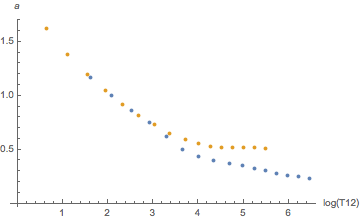
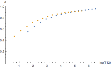
Der einzige Unterschied besteht darin, wie die Ceiling (die momentan minimal erlaubte Tiefe) aus den Gewebesaettigungen $p_i$ berechnet wird: Bühlmann verwendet einen affine Zusammenhang mit dem Umgebungsdruck (die Geradengleichung wird durch die gekannten $a$ und $b$ Koeffizienten parametrisiert. Verwendet man Gradientenfaktoren, die wird Geradengleichung noch weiter modifiziert (abhängig von der maximalen Ceiling, aber die Ceiling, geplottet als Funktion von $p_i$ bleibt eine Gerade, ist also affin).

Für VPM-B ist dies anders: Nur in der nullten Näherung bleibt es eine Gerade: In der Tat wird die Ceiling einfach durch einen konstanten Gradienten (die Differenz zwischen Umgebungsdruck und Gewebedruck) gegeben, dieser ist sogar von der Tiefe unabhängig:

$$p_{amb} – p_i \le G_{0,i}.$$

Dieser Gradient wird als Anfangsgradient $G_0$ bezeichnet. In dieser Näherung verhält sich VPM-B genau wie ein Buehlmannmodell mit modifizierten a und b Koeffizienten.

Für die nächste Näherung, die “Boyle-Kompensation” müssen wir etwas über Blasen wissen. Alles, was wir brauchen, ist, dass diese eine Oberfläche haben und dass die Oberfläche zur Gesamtenergie proportional zu ihrer Fläche beiträgt:

$$E_{surf}= \gamma r^2$$

für eine Blase mit Radius $r$ (wir können numerische Faktoren wie $4\pi$ in der Proportionalitätskonstantante $\gamma$ absorbieren). Die Kraft auf die Oberfläche, die diese zu verkleinern sucht, ist dann

$$F_{surf} = \frac{\partial E_{surf}}{\partial r} = 2\gamma r.$$

Diese Kraft wirkt auf die gesamte Fläche, teilen wir durch den Flächeninhalte erhalten wir einen Beitrag zum Druck in der Blase:

$$G=\frac{2\gamma}r.$$

Derartige Formeln, bei denen eine Blasenoberfläche $2\gamma/r$ zum Druck beiträgt, werden im Folgenden immer wieder auftauchen.

Insbesondere zu dem Zeitpunkt im Tauchgang mit der tiefsten Ceiling ist der Gradient $G_0$ genau dies. “Boyle-Kompensation” bedeutet, dass der von nun an tiefenabhängige Gradient (also der Umgebungsdruck minus Gewebedruck) dadurch gegeben ist, dass man eine Blase nach dem Boyle-Marriott-Gesetz expandieren lässt, also dass man annimmt, dass $pV$ konstant ist. $p$ im Inneren der Blase (was nach dem Modell mit dem Gewebedruck gleich ist) wird dann berechnet als der Umgebungsdruck plus dem momentanen maximalen Gradienten. Das Volumen der Blase ist proportional zu $r^3$ und dies ist nach der obigen Formel proportional zu $1/G^3$. Alles in allem ist die erlaubte Differenz zwischen Gewebe- und Umgebungsdruck in der Tiefe $d$ gegeben durch die Lösung von

$$\frac{G+p(d)}{G^3} = \frac {G_0+p_{1st\ ceiling}}{G_0^3}.$$

Folglich ist der der maximale Gradient keine Gerade mehr, sondern die Lösung einer kubischen Gleichung (für die wir in Subsurface auch einen analytischen Ausdruck verwenden statt wie im Originalcode eine Nullstellensuche mittels Newtonverfahren zu veranstalten).

Ich habe noch nicht erklärt, wie der Anfangsgradient $G_0$ berechnet wird. Für VPM-B lautet der Ausdruck dafür

$$G_0 = 2 \frac\gamma{\gamma_c} \frac {\gamma_c – \gamma}{r_{reg}}.$$

Hier ist $r_{reg}$ der “Crushing-Radius”, der sich mittels

$$\frac{2(\gamma_c-\gamma)}{r_{reg}} = p_{max} + \frac{2(\gamma_c-\gamma)}{r_{crit}}$$

aus der Oberflächenspannung der Blase berechnen lässt.

Hier wiederum sind $\gamma$ und $\gamma_c$ Oberflächenspannungen (am Ende: Modellparameter), ebenso wie $r_{crit}$. Letzteres ist der Parameter, an dem man den Konservatismus des Modells einstellen kann: Jede zusätzliche Konservatismusstufe (zum Beispiel VPM-B+3) erhöht $r_{crit}$ um 5 Prozent. $p_{max}$ ist das Maximum des Umgebungsdrucks während des Tauchgangs. Im Prinzip soll man diesen auch wieder exponentiell an $r_{crit}$ angleichen; dies kann man aber getrost ignorieren, da die Halbwertzeit von zwei Wochen viel länger als alle relevanten Zeitskalen eines Tauchgangs sind.

Jetzt haben wir alles, was wir brauchen, um eine Deko-Profil zu berechnen: Für jede Tiefe kennen wir wie im Buhlmann-Modell den maximal erlaubten Überdruck.

Es stellt sich heraus, dass die so erhaltenen Dekoprofile viel zu lange dauern. Hier kommt der “Kritische-Volumen-Algorithmus” ins Spiel. Wir erhöhen leicht den Anfangsgradienten (bisher war das $G_0$ und unterwerfen den dann ebenso der Boyle-Korrektur.

Die Idee dabei ist, dass der Körper eine bestimmte zusätzliche Menge an Gas in Blasenform verträgt. Dieses erlaubte Volumen ist wiederum ein Modellparameter und wird mit einem wie folgt für einen Anfangsgradienten $G_0′$ berechnet: Es wird angenommen, dass es vor dem Tauchgang eine bestimmte Verteilung der Blasenzahl abhängig von ihrer Größe im Körper gibt. Dadurch, dass der Anfangsgradient von $G_0$ auf $G_0′$ erhöht wird, erhöht sich die Zahl der wachsenden Blasen (generell wachsen grosse Blasen, da bei ihnen der Druckanteil durch die Oberflächenspannung kleiner ist, siehe oben, während kleine schrumpfen). Die Zahl der zusätzlich wachsenden Blasen ist dann in linearer Näherung proportional zu (und dies ist einer der Orte, wo ich die Herleitung nicht verstehe, aber verwenden wir den Ausdruck trotzdem):

$$\frac{G_0′-G_0}{G_0′-\alpha G_{crush}}.$$

Hier ist $\alpha$ ein weiterer Modellparameter und $G_{crush}$ ist der maximale Überdruck des Umgebungsdrucks zum Gewebedruck während des Tauchgangs und nach den Regeln des Modells ebenso der maximale Unterschied zwischen dem Innen- und dem Außendruck einer Blase (wenn dieser zu groß ist, kommen wir ins “nichtpermeable Regime” und man wendet eine weitere Boyle-Kompensation an).

Eine weiter Annahme ist, dass die Rate mit der Gas in die Gasphase in Blasen geht, proportional zum Gradienten $G_0′$ ist (die erfolgte Boyle-Compensation fällt hier unter den Tisch). Da man also annimmt, dass der Gradient während der Deko (definiert als die Zeit, zwischen dem Zeitpunkt, bei dem das erste Gewebe beginnt, den Gewebedruck wieder abzubauen bis zum Erreichen der Oberfläche) konstant ist, multiplizieren wir den Gradienten mit der Dekozeit (dies ist die Zeit $t_D$ die wir oben berechnet haben, als wir den Dekoplan aus den Gradienten berechnet haben).

Sobald wir die Oberfläche erreichen, gibt es immer noch einen Überdruck im Gewebe, zunächst $G_0′$ (wiederum wird die Boyle-Kompensation unterschlagen) und im Folgenden fällt dieser exponentiell entsprechend der obigen Diffusionsgleichung auf 0. Somit ist das Zeit-Integral des Gradienten an der Oberfläche $G_0’/\alpha_i$. Nimmt man alles zusammen, ist das Kriterium für den neuen Gradienten $G_0′$

$$V\ge \frac{G_0′-G_0}{G_0′-\alpha G_{crush}} G_0′ \left(t_D +\frac 1{\alpha_i}\right)$$

Dies löst man nach $G_0′$ auf, was dann für einen neuen Dekoplan benutzt wird, der wiederum ein neues $t_D$ ergibt. Dieses Verfahren wiederholt man, bis sich $G_0′$ nicht mehr ändert.

Bis auf etwas Kleingedrucktes (wie etwa wie der Dekoplan aus dem Gradienten im Detail berechnet wird) ist dies der gesamte VPM-B Algorithmus. Mit diesen Informationen kann man ihn im Prinzip selber implementieren.

In einem zukünftigen Post plane ich dann die Physik anzusehen, die aufgerufen wird, um die hier verwendeten Gleichungen herzuleiten.