When the Subsurface mailing list recently received the request if the planner could implement the DCIEM model as well my first reaction what “Whut?” has I had not heard of it before.
Turns out, DCIEM stands for “Defense and Civil Institute of Environmental Medicine” which was a research institution of the Canadian military and is now part of DRDC Toronto according to Wikipedia. The request to Subsurface was apparently prompted by the fact that Shearwater announced to implement the model into their dive computer for commercial divers. The “for commercial divers” sounds to me like this is more to tick some boxes in the health and safety requirements for these people rather than something that the diving world at large should adopt. But still, it might be interesting to see what this model actually does.
Some googling suggests that this model is mainly consumed not in terms of an algorithm in planning software or dive computers but in the for of tables. A 1992 version can for example be found here.

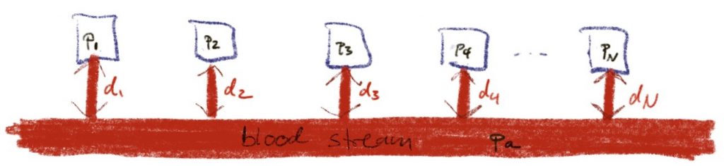
But Google also finds a review paper by Nishi and Tikuisis that explains that the DCIEM model is a non-linear model developed by Kidd and Stubbs. It shows as four compartment discretisation of a slab of tissue together with a ODE for time evolution:
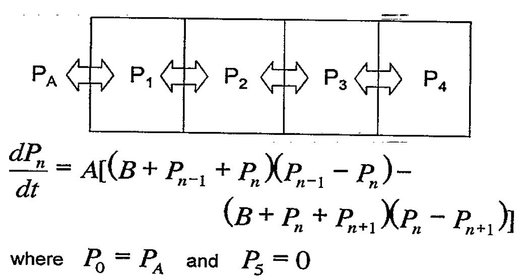
As written, I cannot make much sense of it but things clear up when the expression is expanded:
\(\dot p = ab \Delta p +a\Delta p^2\)Here, p is the vector of tissue pressures and Δ is the discrete Laplacian that for a sequence (s) is
\( \Delta s_{n} = s_{n-1} -2 s_n + s_{n+1}.\)If there were only the first term on the RHS, that would simply be a diffusion equation that I would also have written if somebody had asked me to write down a model for a slab of tissue. I have no clue where the second, non-linear term comes from but clearly it can safely be ignored as long as p<<b. There is also a paper by Nishi and Kuehn that gives a FORTRAN implementation of the model (doesn’t this sound familiar…). In the source code, I find a value of b=274.5 which is supposedly in units of psi which translates to 19bar, so the non-linear term should will not be relevant for anyone with a depth limit short of 200m. In the review paper it is stated that the constants of the model were fitted to bubble measurements after trial dives but one could wonder how this is would be possible unless compartment pressures at least came near to 20bar…
The paper with the FORTRAN program also explains that the relation between tissue pressure and ambient pressure is pretty much a standard \(p_{amb}\ge c_1 p_{tissue} + c_2.\)
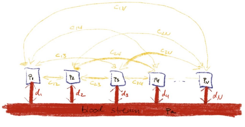
More interesting is that the discretised slab is an example of the interacting tissue models I talked about in the post about those being equivalent to independent tissues. For four tissues, the discretised Laplacian (there is of course also a closed form) has eigen values \(\frac{-3\pm \sqrt 5}{2}, \frac{-5\pm\sqrt 5}{2}\) which numerically range between -3.6 and -0.38.
So, the four independent tissues after diagonalization cover one decade of half-times all proportional to 1/ab.
So, taking everything into account, the DCIEM model is (equivalent to) a Bühlmann type model with four tissues coving a somewhat small range of half-times. So I would expect with an appropriate choice of constants, one can produce somewhat reasonable deco schedules at least for air dives (we have not discussed different gases) with not too long runtimes. But a full blown Bühlmann (possibly with gradient factors) is much more expressive.