Can we calculate no-fly-times?

There are various recommendations how long one should not fly after surfacing from a dive. DAN has recently done a study where they did Doppler measurements on a plane and recommends an interval of 12 hours after a single dive and 24 hours after repetitive diving.

But one would think that it should be possible to use a decompression model that works well under water to compute such a time. So let’s do this in this post or at least compute a conservative estimate. To be specific, we will use the Buhlmann model. We do that calculation compartment by compartment and assume that when leaving the water, the tissue has the maximally allowed partial pressure for surfacing (i.e. this tissue was the guiding tissue for the final part of the ascent). Clearly, this is a conservative assumption. Then, according to the model

\(p_s = (p_i -a)b.\)

Here, ps is the surface pressure and a and b are the usual Bühlmann coefficients.

Then we do a surface interval (whose length we wish to determine in the end) during which the partial pressure decays exponentially:

\(p_i(t) = f_{N_2} p_s+ (p_i(0) – f_{N_2}p_s)e^{-\gamma t}\)

where f is the N2 fraction the the breathing gas (0.79 for air which we are probably breathing while waiting for the plane to board). Finally, we don’t want the cabin pressure to be less than the minimal ambient pressure that Dr. Bühlmann recommends. We want to parametrize the cabin pressure using the barometric formula which asserts (assuming constant temperature) that the pressure drops exponentially at height with decay constant that the pressure is 1/e at about hs=8500m above sea level. So, we set

\(e^{-h/hs} p_s= (p_i(t) -a)b.\)

This we can then solve for t. Actually, being conservative, we want to throw in gradient factors. Again, being conservative, we don’t further linearly extrapolate gradient factors, but will use GFhi everywhere on the surface. Plugging everything in (with the help of Mathematica and some manual massaging) we find

\(e^{\gamma t} = \frac{a GF/p_s + 1-f_{N_2} + GF(1/b -1)}{a GF/p_s – f_{N_2} +e^{-h/h_s}(1+GF(1/b-1))}.\)

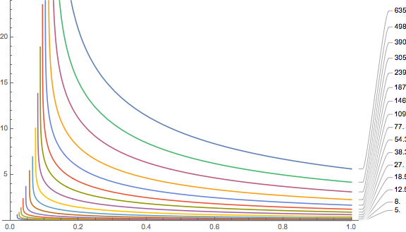
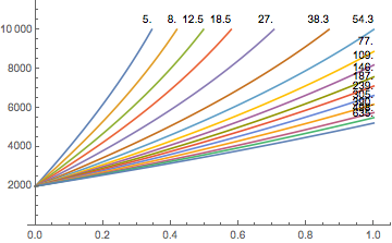
Now, we have to plug in numbers. For the cabin pressure, according to Wikipedia, we will assume h=2400m for older aircrafts. The wait times (in hours) for the different compartments are then shown in this plot:

No-fly-times in hours for different compartments plotted against gradient factor. The labels are the tissue half-times in minutes.

You are supposed to see a number of things:

  • The waiting time depends strongly on which tissue we are dealing with. For reasonably large gradient factors, only the tissues with half-times of several hours contribute significant waiting times. Remember, for this calculation, we assumed the loading is at its maximal value when you get out of the water. For realistic sports/tec-diving scenarios (as opposed to saturation diving) that should be quite hard even on a weeklong liveaboard  with at least five dives a day. If slightly faster tissues are leading, the inferred no-fly times are much shorter, probably shorter than the queue at check-in. I looked at some data from real dive trips where people got everything out of their booked liveaboard but they got nowhere close to exciting the slow tissues. In the Subsurface planner I had to do five consecutive 2-hour dives with less than two hour surface interval to see at least some ceiling for the 239 minute compartment. In the plots, this has the blue line and leads to a no-fly time of much less than 5 hours.
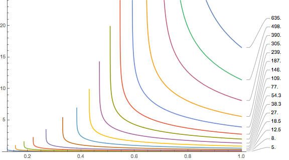
  • The plot ends on the left (small gradient factors) with diverging values. These divergences move to higher gradient factors when you increase the cabin pressurisation equivalent altitude (for example by assuming a loss of cabin pressure, remember this is when the oxygen masks are supposed to drop from the ceiling)
    Same plot with 4500m of altitude

    This comes about as the no-fly time becomes infinite or even complex as according to the Bühlmann-with-gradient-factors limit, your are not allowed to be at the ambient pressure at that altitude even when saturated with the nitrogen that you experience at sea level. We can compute this limiting altitude by solving
    \(f_{N_2} p_s = e^{-h/h_s} p_s (GF/b-GF +1) + a GF /p_s\)
    for the altitude via
    \(e^{-h/h_s} = \frac{f- aGF/p_s}{GF/b -GF +1}.\)
    This is shown here, the maximum altitude after waiting an infinite amount of time:

    Maximal altitudes in meters for the different compartments as a function of the gradient factor.


  • All these calculations are for air (or nitrox underwater since all we used was the assumption that the nitrogen saturation is at the limit). In particular, in view of an earlier post (N2 vs. He, what’s the difference?) there should not be large differences.
  • You could try to repeat the same argument for VPM-B but according to that model, if you followed it during the ascent, the no fly time would always be infinite: The ascent is determined such that when you surface and stay at ambient pressure, you will just create the maximum amount of free gas that is barely allowed. So going to any altitude and lowering the ambient pressure further would release more free gas than allowed, no matter how long you waited. The only way out would be to produce fewer bubbles on the earlier ascent while still in the water, then you would have some reserves to go to altitude.

What are we supposed to conclude from this? One takeaway message is waiting for the recommended 24 hours is not totally off, in particular if there is a chance that your very slow tissues have loaded a significant amount of nitrogen.

On the other hand, for realistic dives, 24 hours is likely on the very conservative side. At least from the perspective of decompression theory. From this perspective it is a total mystery to my what kind of reasoning dive computers use to determine a no-fly time.

Apart from these model considerations, DCS symptoms often enough do not show up immediately after a dive but up to several hours later. And when you are in that situation that you find yourself with DCS symptoms (even those that would have occurred irrespective of flying or not) your chances for immediate proper treatment are probably much higher if you are not confined to an aircraft above the middle of the ocean. So even from that perspective it makes sense to wait a bit more to make sure you will not need a chamber in the next few hours.

PS: If you want to play around with the formulas, here is my Mathematica notebook.

More confusion from Isobaric Counter Diffusion

After I expressed my worries about the commonly used criterium for the occurrence of Isobaric Counter Diffusion (ICD), namely a gas change in which the N2 fraction increases by more than a fifth of the drop in the He fraction, I learned (suggested by the OSTC source code, around lines 2220) about another (and much better motivated) criterium: Simply check if the leading tissue is taking up more N2 than it dumps He to the environment. That would mean that the net effect is an on-gassing of inert gases.

\(\Delta p_{He}<0,\quad \Delta p_{N_2}>0,\quad \Delta p_{He} + \Delta p_{N2} >0\)

This sounds reasonable: If this is true for the leading tissue, the decompression is ineffective as the total inert gas pressure goes up.

So I implemented it in Subsurface. Turns out, this does not trigger where you expect it. For example for a 60m dive with 20min of bottom time on 18/45, forcing a gas change to air (i.e. high N2) at 45m does not trigger it: Yes, He in the tissue goes down and N2 goes up but He is so much faster that the net effect is still off-gassing.

But for the same dive, it triggers at a different, unexpected place: At the beginning of the ascent (at 58m to 54m). How does this come about? At the end of the bottom time (and also during the start of the ascent), the leading tissue is the second (with 8min of N2 half-time). After 20min bottom time, He is almost saturated but N2 still has a way to go. Thus, at the start of the ascent, pretty much off the bottom, He starts off-gassing while for N2, the depth difference is not really noticeable, so it is still on-gassing with positive net. So there actually is counter diffusion even without a gas change!

I guess, nobody would suggest that leaving the bottom at 60m would be dangerous. But this seems to be the only place where counter diffusion actually happens!

I tend to believe more and more that this whole ICD story is either not explained at all by a diffusion model (maybe because it is only relevant in the inner ear that does not follow this simple tissue+environment model) or it is totally bogus.

So I would like to hear from you, dear readers, do you have any experiences with ICD or could you suggest a dive profile where it should be relevant?

Isobaric Counter Diffusion Criteria

I would like to hear your opinion about isobaric counter diffusion (ICD) and the criteria you apply to decide if a gas switch should be considered dangerous.

But first a bit of background to make sure we are all on the same page: ICD is the phenomenon that occurs when you switch from a mix with a lot of helium to a mix that contains less helium but more nitrogen. Then it can happen (depending on the tissue loading) that some tissue is off-gassing He but on-gassing N2, i.e. that the two inert gases move in opposite directions. And historically this is considered bad for your deco.

As the He atoms are much small than the N2 molecules the former diffuses faster than the latter so, in typical situations, in total the off-gassing should happen on a shorter timescale than the on-gassing and thus the net effect will be that the tissues inert gas loading goes down. Anyway, this effect should be covered by the usual diffusion based deco algorithm (as this is exactly what it simulates) and no additional care would need to be taken as long as the diver stays within the boundary of the deco algorithm.

There is, however, an argument due to Steve Burton that suggests to take the solubility of the gases (in typical tissue) into account to compute the absolute amount of inert gases in the body. And since that is about 5 times higher for N2 than for He, he argues that in order to have a net unloading of the absolute amount of gas one has to limit the change in N2 percentage in the breathing gas by 1/5 of the change in He percentage in the breathing gas.  And at least one technical diving school of teaching seems to have adopted this criterium.

We are currently discussing if we implement this check into Subsurface and warn the user if a gas switch violates this “rule of fifth”. I am not sure though if I buy into this line of thought. After all, everything we do in deco planning is based on partial pressures, we never consider the absolute amount of gas. It is the partial pressure that plays the role of the fugacity determining if a particle moves across the diffusion boarder (in or out of the tissue say) and the rate is proportional to the differences (this is the mantra of diffusion based decompression models). So the solubility and with it the total amount of gas should play no direct role. I wonder if this rule of fifth (as is seems it comes out of a theoretical consideration with questionable initial assumptions) has received any empirical evaluation. Note that for example it forbids to change from Tx18/45 directly to EAN50 (as He goes down by 45% of which a fifth is 9% while the N2 fraction increases by 13 percentage points, more than 9%) even though I understand this is rather commonly done.

There is another ICD theory investigated by Doolette and Mitchell that focusses on inner ear DCS. They argue that in the inner ear the common diffusion model assumptions are violated since there is a relatively large amount of inner ear liquid that is not in direct (diffusive) contact with them ambient pressure (blood in practice) but only indirectly via inner ear tissue. So all off-gassing of the liquid goes first into the tissue. So what happens in an ICD caused inner ear DCS accident is that while that tissue is already on-gassing N2 from the environment (=blood) it is still receiving the He that comes out of the liquid and therefore experiences an over all uptake in inert gas which eventually causes DCS.

But i have not seen any hard “you should avoid doing the following” criterion that is derived from this line of thought beyond a general “shouldn’t really be a problem when using a CCR and otherwise be careful and always maximise the O2 fraction within the boundaries set by MOD”.

So, for the deeper trimix divers here: How do you decide which gas switches are ok and do you want your dive planning software to warn you about those.

PS: A last warning: It makes no sense to think about ICD in a way like “stuff moves in different directions, so the in-moving particles clog the out-going ones” as this little thought experiment shows: There are two stable nitrogen isotopes N-14 and N-15 (the former much more common in nature) that are chemically not distinguishable (only for example in a mass spectrometer). Image you are breathing a nitro mix with only N-14. Then you switch to the same mix but with all the N-14 replaced by N-15. Then there will be a counter diffusion of N-14 vs N-15. But of course, since both are chemically equivalent there are absolutely zero physiological consequences even, so the argument that the in-moving N-15 clogs up the out-moving N-14 cannot hold (and so it cannot hold in the case above).

VPM-B for real dives (or not)

The VPM-B model (of which I have described my understanding in previous posts) has a “derivation” in terms of bubble physics which I, as readers should have noticed, have some trouble to follow through completely as it is, to say the least, ad hoc and sketchy in places. I bet, only based on this derivation in prose plus formulas, nobody would be able to write a program to compute a VPM-B deco plan.

But we are lucky: There is a reference implementation in terms of a FORTRAN program. So, even though the VPM-B code in Subsurface is a complete rewrite (and solves many things algorithmically differently than the original code), we did a lot of testing to make sure that the plans we produce are identical to the plans computed using the FORTRAN program, even in places where we thought it makes little sense (like starting the ascent to the next stop when the ceiling depth equals the depth of the next stop rather than starting a bit earlier and making sure never to violate the ceiling during the ascent to the next stop (which is different since the ceiling goes up during the time it takes to get to the next stop). The latter is, at least to me, better motivated physically (“simply never violate the ceiling”) than basing the stop time on what happens at a different depth (namely the next stop depth) and we use the latter when computing Bühlmann schedules. But for VPM-B, we thought, given that we do not really understand the physics, we should not modify the model based on physics.

I have talked in the past about the Bühlmann model not being well defined to make all implementations come up with identical plans. In a sense, we are in a better situation with VPM-B, since there is the FORTRAN program which (at least for us) defines the model. But the problem is: This definition works only for the situation that you can compute with the FORTRAN program: You specify the bottom part of the dive and then let the program work out the ascent. Strictly speaking there is no definition for real dives: Dives where the distinction between bottom part and deco is blurred. But this is exactly what you have if you were to implement it in a dive computer or, as for Subsurface: Implement it in a dive log to show a ceiling for a logged dive (after all, Subsurface is mainly a divelog). For real dives, you cannot tell the exact point where bottom time ends and deco begins.

Unfortunately, the model depends on this: As explained in the VPM-B derivation post, one parameter that goes into the computation is the total deco time \(t_D\) (clearly that ends when you reach the surface, but where does it start?) but there are other parameters that you are supposed to evaluate at the beginning of the ascent like \(p_{1st ceiling}\) and the initial gradient for the Boyle compensation. All this depends on the time you call the end of bottom time and thus the computed ceilings also depend on that.

For Subsurface, we decided to take the point of time with the deepest ceiling (which, strictly speaking, is a circular definition but in practice is irrelevant) as the end of bottom time and base the ceiling computation in logbook mode on that. But that, to some degree, is arbitrary. And even for dives that we planned using VPM-B (and thus agree with the schedules computed by the FORTRAN program), applying this logic yields a slightly different ceiling. So it can appear that a VPM-B planned dive violates the VPM-B ceiling. But this is only due to the fact that the model is not really defined outside the planning situation.

Or put differently: You need to make arbitrary assumptions (not based on the depth profile and the gas you are breathing) to come up with a VPM-B ceiling. Which, at least for me, doesn’t strengthen my believe into this model.

PS: I am planning to be at the Boot dive show in Düsseldorf on Friday January 26th. If you happen to be there as well, please let me know and we can shake hands!

DIY on the fly

With the new version of Subsurface out today, I would like to point to a feature that was already there in 4.7.4, but which just got more usable: Computing deco variations in the planner.

This is motivated by the discussions about Ratio Deco and Deco On The Fly, for a discussion see this post by Rick. These approaches to computing deco are not really attempting to model anything that is supposed to go on in the diver’s body but simply to take a very pragmatic approach and interpolate deco schedules from known ones. If you like, they are (or attempt to be) mnemonics to learn deco plans by heart. The idea is simply that you memorise a reference plan and also how you have to modify deco if you modify the bottom part of your dive.

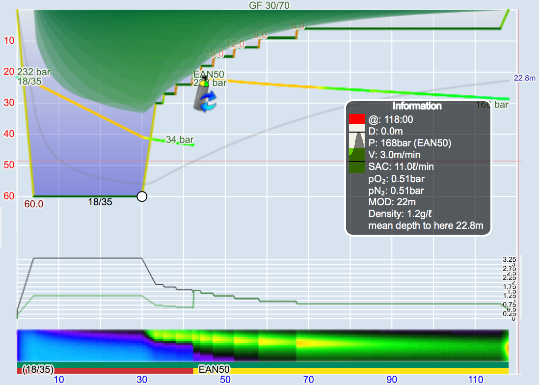
With Subsurface, you can now do exactly this: You can take any dive that you planned in the planner as reference dive and it will tell you how your total deco time depends on the bottom part. Take for example this trimix dive to 60m with 30min bottom time:

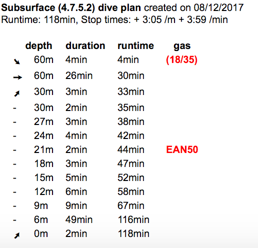
The runtime table says

The important line is the second:

Runtime: 118min, Stop times: + 3:05 /m + 3:59 /min

This tells you how to adjust the total deco time when changing the bottom time (the segment at 30m): For each meter that you go deeper, you have to add about three minutes (for example if you went to 63m for half an hour, you would have to add about 9 minutes or if you only went to 58m you could shorten your deco by 6 minutes). Similarly, if you change the bottom time you have to pay every extra minute on the bottom by about four minutes in deco.

It does not tell you how to distribute this time over the different stops but a good rule of thumb would be to do it roughly proportional to the time you already spend at the stops. So for example, of the about 90min of total deco time you spend roughly half at 6m,  you would also add half of the extra time at this last stop.

These numbers are supposed to be something like the partial derivative of the total deco time with respect to depth and duration of the bottom time element (actually: the last manually entered part of the dive). You are supposed to multiply these derivative with the actual variation of the bottom segment that you do.

How do we compute these numbers? When this calculation is enabled, Subsurface actually computes five extra plans: It first computes the original plan, but now with second resolution of the stops instead of minute resolution. Then it shortens the bottom segment by one minute and computes the plan (again to seconds) and then computes a plan for a bottom time extended by one minute. Then it computes to more plans for one meter shallower and one meter deeper.

This give us two time differences both for depth and duration variations. What is displayed is the average of those. But a bit of experimentation shows that the difference is typically only a few seconds (and what are seconds for 90min deco?). This is also a measure how good this linear approximation is (as this the quadratic correction): It gives me confidence to say this approximation isn’t too bad for a few minutes or a few meters.

So having these two numbers also on the runtime table should give the diver much more confidence in how to react to unforeseen changes of plan (both shallower and deeper and shorter and longer). But of course, always remember: Plan the dive, dive the wreck, wreck the plan!

CCR Schreiner Equation

Since there was a question on Scuba Board about how to compute the tissue pressures when diving a CCR (i.e mainlining constant partial pressure of oxygen) when changing depth at a constant rate. When putting this on a computer I would say doing it for small time steps and pretending to be at constant depth for that short amount of time doesn’t do much wrong and you will end up doing this anyway (at least that’s what we do in Subsurface). But for the fun of it, let’s work out the analytic solution.

Let’s start by figuring out the inert gas ambient pressure at a given depth. We call \(p_d\) the diluent partial pressure, \(p_{O2}\) the partial pressure supplied from the oxygen cylinder (note that this is not the oxygen partial pressure since there is going to be some oxygen in the diluent as well), \(d\) is the depth, \(f_{O2}\) is the fraction of oxygen in the diluent while \(f_i\) is the fraction of the inert gas we are computing in the diluent.

There are two obvious equations: The ambient pressure is equal to the diluent pressure plus the oxygen pressure in the loop:

$$ p_d + p_{O2} = p_a = p_{surf} + dg\rho$$

Here, \(p_{surf}\) is the surface pressure, and \(\rho\) is the density of water and thus \(g\rho\) the conversion factor between depth and pressure. The second equation says that the total partial pressure of oxygen (from diluent and oxygen cylinder combined) has to equal the set point pressure \(p_s\):

$$f_{O2} p_d + p_{O2} = p_s.$$

We can subtract both equations to eliminate \(p_{O2}\) and find

$$ p_d = \frac{p_{surf} + g\rho d -p_s}{1-f_{O2}}.$$

This goes into the usual diffusion equation for the inert gas loading in the tissue \(p_t\) that we are ultimately interested in:

$$\dot p_t = -\gamma( p_t -f_i p_d).$$

\(\gamma\) is the usual diffusion constant that is related to the inverse of the tissue half-time by a factor of \(\ln(2)\). Finally, we want the depth to change linearly in time, so \(d=d_0+vt\) where my sign convention is that \(v\) is the descend velocity, make it negative for ascends.

So we have to solve a linear inhomogeneous ODE with constant coefficients which we could tackle by “varying the constants”, but of course we are lazy and let Mathematica do the job. After a bit of massaging, we find

$$p_t = \frac{f_i}{1-f_{O2}} \left( e^{-\gamma t} -1\right) \left( p_s + \frac{vg\rho}\gamma\right) + e^{-\gamma t}\left( p_0 – \frac{f_i}{1-f_{O2}} (p_{surf} + d_0g\rho)\right) + \frac{f_i}{1-f_{O2}}(p_{surf} + dg\rho)$$

where \(p_0\) is the initial tissue loading. So, here you go this is the CCR Schreiner equation. Or, if you want to follow the tradition to attaching names to simple solutions of ODEs, I allow you to call it the Helling equation.

Update: If you are worried that a constant water vapour pressure has not been taken into account, you can bring it in by replacing the set point by the actual set point plus the water vapour pressure in all equations above.

We moved

Finally,  The Theoretical Diver is on its own domain thetheoreticaldiver.org . I had intended this move for a long time but it became necessary as the ancient WordPress instance had uninvited visitors (don’t get me started on why it was impossible to update that beyond mentioning that the OS version of the host of that blog required me to run a very old Debian release which came with an old PHP version which only allowed a WordPress version from about the time when my grandma went to elementary school).

So here we are now. And since WordPress does not really like to be moved to a new domain (yes, they store absolute paths in their database, no clue why) and backing up the old was also difficult given how old the WP version was (which excluded most plug-ins) I moved all posts essentially bu cut&paste. I tried to update all the links as well. But please let me know if you find something outdated.

What I couldn’t move are the comments. Which is a pity.

So, once more, welcome to the new site! I hope you feel at home.

VPM-B: How to compute your deco

This is the first technical post about the inner workings of the VPM-B deco model. Here I will just present the algorithm (including the relevant formulas, some of them maybe in an unusual form) while the physical motivation or derivation will be the subject of a future post.

I try not to parrot the original explanations (which, honestly, I do not really understand) but rather put in words what I learned by staring long enough at the subsurface implementation of the model. As I explained earlier, we tried to make this an independent implementation but of course in the end we made sure it produces the identical deco schedules to the original FORTRAN code (that we took as the definition of the model).

First of all, it is not that different from the Bühlmann model, it rather builds on it. For the sake of presentation, I will assume you are familiar with how that model works (if not, I wrote a brief summary with some background in German, to be translated to English soon). In particular, it computes the same tissue loadings with inert gases following a simple diffusion equation

$$\frac{dp_i}{dt} = \alpha_i(p_{amb}-p_i)$$

where the time constant \(\alpha_i\) is essentially the inverse tissue half-time.

The only difference is how to compute the current ceiling for a snapshot of tissue loadings (“tensions” in the deco theory speak) \(p_i\): Bühlmann proposes an affine dependence on the ambient pressure (with the affine relation given in terms of the famous \(a\) and \(b\) coefficients. If you use gradient factors, this affine relation is further modified (depending on your lowest ceiling), but when you plot the ceiling as a function of \(p_i\) it is still a straight line, i.e. affine.

This is different for VPM-B: Only in the zero’s approximation it is still a straight line. In fact, there the ceiling is simply given by a maximal gradient (difference between tissue pressure and ambient pressure) that is independent of the depth:

$$p_{amb} – p_i \le G_{0,i}.$$

This is called the initial gradient \(G_0\). In this approximation, VPM-B is like Buehlmann, only with different a and b coefficients.

For the next approximation, the “Boyle compensation” we need to know a little bit about bubbles. in fact, the only thing one needs to know is that they have a surface and in the total energy balance of the bubble the surface contributes proportional to its area:

$$E_{surf}= \gamma r^2$$

for a bubble of radius r (we can absorb all kinds of numerical constants like \(4\pi\) in the proportionality constant \(\gamma\). Then the force on the bubble surface that wants to shrink it is

$$F_{surf} = \frac{\partial E_{surf}}{\partial r} = 2\gamma r.$$

Finally, this force acts on all of the surface, by dividing by its area again, we get the surface’s contribution to the pressure

$$G=\frac{2\gamma}r.$$

This type of formula, the a bubble surface contributing to the bubble’s internal pressure by \(2\gamma/r\) you will see over and over again.

In particular, that the deepest point in the dive, or actually when reaching the first ceiling, the gradient \(G_0\) is exactly this. And the Boyle compensation means that the (now depth dependent) maximal gradient (i.e. ambient pressure minus tissue pressure) is given by letting such a bubble expand according to Boyle’s law, i.e. by assuming that \(pV\) is constant. \(p\) inside the bubble (which is supposedly the same as the tissue pressure) is then given by the ambient pressure plus the momentary maximal gradient while the volume is proportional to \(r^3\) which according to the above formula is proportional to \(1/G^3\). So in total, the allowed difference between the tissue and the ambient pressure at depth \(d\) is given by solving

$$\frac{G+p(d)}{G^3} = \frac {G_0+p_{1st\ ceiling}}{G_0^3}$$

So, rather than being a straight line, the maximal gradient is now the solution of a cubic equation (for which, in Subsurface, we use an analytic expression rather than running a Newton root finder as in the original implementation).

So far, I did not tell you what the initial gradient \(G_0\) is. The VPM-B expression for it is

$$G_0 = 2 \frac\gamma{\gamma_c} \frac {\gamma_c – \gamma}{r_{reg}}.$$

Here, \(r_{reg}\) is the crushing radius which is again determined from an expression of a bubble surface tension:

$$\frac{2(\gamma_c-\gamma)}{r_{reg}} = p_{max} + \frac{2(\gamma_c-\gamma)}{r_{crit}}$$

Here \(\gamma\) and \(\gamma_c\) are some surface tensions (effectively parameters of the model) as is \(r_{crit}\). The latter is where one can tune the conservatism of the model: Each level of conservatism (like three levels in VPM-B+3) increases \(r_{crit}\) by 5 percent. \(p_{max}\) is the maximal ambient pressure encountered during the dive. In principle, it is also assumed that over time, \(r_{reg}\) also exponentially approaches \(r_{crit}\) again, but it is totally safe to ignore this since the decay time is supposed two weeks, far too long to play any role at the typical time scales of the dive.

Now, you have everything to compute a deco schedule: Like in the Buehlmann model, you know for each depth what the maximal gradient is.

Turns out, these schedules take far too long. This is where the “critical volume algorithm” comes into play. We now slightly increase the first gradient (the role so far played by \(G_0\)) which then is also subject to the Boyle compensation.

The idea here is that the body can tolerate an additional amount of gas going into bubbles. The maximal volume, again, is a model parameter and it is compared to the excess volume as follows: One assumes there is some distribution of bubble sizes. By enlarging the gradient \(G_0\) to \(G_0′\), the number of additional bubbles will be (this is one of the places where I do not understand the derivation, but let’s take the expression anyway) proportional to

$$\frac{G_0′-G_0}{G_0′-\alpha G_{crush}}.$$

Here, \(\alpha\) is another constant and \(G_{crush}\) is the maximal excess of the ambient pressure over the tissue pressure over the dive which also happens to be the pressure gradient over the surface of the bubble (if that is too big, we are in the “impermeable regime” and then there is another Boyle type compensation).

Furthermore, rate of additional out gasing is assumed to be proportional to the gradient \(G_0′\) (totally ignoring the first Boyle compensation) and the whole thing lasts (assuming a constant gradient) over all of the decompression time (defined as the time from the first tissue starting to release gas again until we reach the surface). This decompression time \(t_D\) is what we computed above where I said we can now compute a deco plan from the gradients.

Once we reach the surface, there is still an overpressure in the tissue compared to the ambient pressure, it starts with \(G_0′\) (again ignoring the Boyle compensation) and then, according to the diffusion equation above, approaches 0 exponentially. so the time integral of the gradient yields \(G_0’/\alpha_i\). Throwing all together, we get as a criterium for the maximal \(G_0′\)

$$V\ge \frac{G_0′-G_0}{G_0′-\alpha G_{crush}} G_0′ \left(t_D +\frac 1{\alpha_i}\right)$$

This we then solve for \(G_0′\) which we can use for computing a new deco schedule which gives a new \(t_D\) and we repeat this until \(G_0′\) does not change anymore.

Apart from some minor fine print (like how in detail the deco schedules are computed) is all there is to VPM-B. With this information, you should, in principle be able to implement it yourself.

In the next post, I will look into the physics that is invoked to argue for some of the expressions that I only quoted here.

VPM-B: Wie funktioniert’s (deutsche Übersetzung)

Dies ist der erste technische Post darüber, wie VPM-B funktioniert. Ich werde nur den Algorithmus beschrieben (mit allen wichtigen Formeln, einige davon vielleicht  in ungewohnter Form), während die physikalische Herleitung in einem späteren Post behandelt werden wird. 

Ich werde nicht versuchen, die ursprüngliche Herleitung nachzubeten (auch schon alleine, weil ich sie nicht wirklich verstehe), sondern vielmehr beschreiben, was ich durch langes Starren auf unsere Implementierung des Modells in Subsurface gelernt habe. Wie vorher schon erklärt haben wir versucht eine unabhängige Neuimplementierung zu machen, haben aber natürlich sicher gestellt, dass die Austauschpläne des ursprünglichen FORTRAN-Programms reproduziert werden. Dieses haben wir letztendlich als die Definition von VPM-B hergenommen.

Zunächst ist dieses dem Bühlmannmodell sehr ähnlich und baut darauf auf. Für diesen Post nehme ich an, dass dieses bekannt ist (falls nicht habe ich hier mal eine kurze Zusammenfassung aufgeschrieben). Insbesondere werden die Sättigungen der verschiedenen Gewebe mit Inertgasen mit der gleichen einfachen Diffusionsgleichung beschrieben:

$$\frac{dp_i}{dt} = \alpha_i(p_{amb}-p_i)$$

wobei die Zeitkonstante \(\alpha_i\) im wesentlichen der Kehrwert der Halbwertzeit des Gewebes ist. 

Der einzige Unterschied besteht darin, wie die Ceiling (die momentan minimal erlaubte Tiefe) aus den Gewebesaettigungen \(p_i\) berechnet wird: Bühlmann verwendet einen affine Zusammenhang mit dem Umgebungsdruck (die Geradengleichung wird durch die gekannten \(a\) und \(b\) Koeffizienten parametrisiert. Verwendet man Gradientenfaktoren, die wird Geradengleichung noch weiter modifiziert (abhängig von der maximalen Ceiling, aber die Ceiling, geplottet als Funktion von  \(p_i\) bleibt eine Gerade, ist also affin).

Für VPM-B ist dies anders: Nur in der nullten Näherung bleibt es eine Gerade: In der Tat wird die Ceiling einfach durch einen konstanten Gradienten (die Differenz zwischen Umgebungsdruck und Gewebedruck) gegeben, dieser ist sogar von der Tiefe unabhängig:

$$p_{amb} – p_i \le G_{0,i}.$$

Dieser Gradient wird als Anfangsgradient  \(G_0\) bezeichnet. In dieser Näherung verhält sich VPM-B genau wie ein Buehlmannmodell mit modifizierten a und b Koeffizienten.

Für die nächste Näherung, die “Boyle-Kompensation” müssen wir etwas über Blasen wissen. Alles, was wir brauchen, ist, dass diese eine Oberfläche haben und dass die Oberfläche zur Gesamtenergie proportional zu ihrer Fläche beiträgt:

$$E_{surf}= \gamma r^2$$

für eine Blase mit Radius \(r\) (wir können numerische Faktoren wie \(4\pi\) in der Proportionalitätskonstantante \(\gamma\) absorbieren). Die Kraft auf die Oberfläche, die diese zu verkleinern sucht, ist dann

$$F_{surf} = \frac{\partial E_{surf}}{\partial r} = 2\gamma r.$$

Diese Kraft wirkt auf die gesamte Fläche, teilen wir durch den Flächeninhalte erhalten wir einen Beitrag zum Druck in der Blase:

$$G=\frac{2\gamma}r.$$

Derartige Formeln, bei denen eine Blasenoberfläche  \(2\gamma/r\) zum Druck beiträgt, werden im Folgenden immer wieder auftauchen.

Insbesondere zu dem Zeitpunkt im Tauchgang mit der tiefsten Ceiling ist der Gradient \(G_0\) genau dies. “Boyle-Kompensation” bedeutet, dass der von nun an tiefenabhängige Gradient (also der Umgebungsdruck minus Gewebedruck) dadurch gegeben ist, dass man eine Blase nach dem Boyle-Marriott-Gesetz expandieren lässt, also dass man annimmt, dass \(pV\) konstant ist. \(p\) im Inneren der Blase (was nach dem Modell mit dem Gewebedruck gleich ist) wird dann berechnet als der Umgebungsdruck plus dem momentanen maximalen Gradienten. Das Volumen der Blase ist proportional zu \(r^3\) und dies ist nach der obigen Formel proportional zu \(1/G^3\). Alles in allem ist die erlaubte Differenz zwischen Gewebe- und Umgebungsdruck in der Tiefe \(d\) gegeben durch die Lösung von

$$\frac{G+p(d)}{G^3} = \frac {G_0+p_{1st\ ceiling}}{G_0^3}.$$

Folglich ist der der maximale Gradient keine Gerade mehr, sondern die Lösung einer kubischen Gleichung (für die wir in Subsurface auch einen analytischen Ausdruck verwenden statt wie im Originalcode eine Nullstellensuche mittels Newtonverfahren zu veranstalten).


Ich habe noch nicht erklärt, wie der Anfangsgradient \(G_0\) berechnet wird. Für VPM-B lautet der Ausdruck dafür

$$G_0 = 2 \frac\gamma{\gamma_c} \frac {\gamma_c – \gamma}{r_{reg}}.$$

Hier ist  \(r_{reg}\) der “Crushing-Radius”, der sich mittels

$$\frac{2(\gamma_c-\gamma)}{r_{reg}} = p_{max} + \frac{2(\gamma_c-\gamma)}{r_{crit}}$$

aus der Oberflächenspannung der Blase berechnen lässt.

Hier wiederum sind  \(\gamma\) und \(\gamma_c\) Oberflächenspannungen (am Ende: Modellparameter), ebenso wie \(r_{crit}\). Letzteres ist der Parameter, an dem man den Konservatismus des Modells einstellen kann: Jede zusätzliche Konservatismusstufe (zum Beispiel VPM-B+3) erhöht \(r_{crit}\) um 5 Prozent.  \(p_{max}\) ist das Maximum des Umgebungsdrucks während des Tauchgangs. Im Prinzip soll man diesen auch wieder exponentiell  an  \(r_{crit}\) angleichen; dies kann man aber getrost ignorieren, da die Halbwertzeit von zwei Wochen viel länger als alle relevanten Zeitskalen eines Tauchgangs sind.

Jetzt haben wir alles, was wir brauchen, um eine Deko-Profil zu berechnen: Für jede Tiefe kennen wir wie im Buhlmann-Modell den maximal erlaubten Überdruck.

Es stellt sich heraus, dass die so erhaltenen Dekoprofile viel zu lange dauern. Hier kommt der “Kritische-Volumen-Algorithmus” ins Spiel. Wir erhöhen leicht den Anfangsgradienten (bisher war das \(G_0\) und unterwerfen den dann ebenso der Boyle-Korrektur.

Die Idee dabei ist, dass der Körper eine bestimmte zusätzliche Menge an Gas in Blasenform verträgt. Dieses erlaubte Volumen ist wiederum ein Modellparameter und wird mit einem wie folgt für einen Anfangsgradienten \(G_0′\) berechnet: Es wird angenommen, dass es vor dem Tauchgang eine bestimmte Verteilung der Blasenzahl abhängig von ihrer Größe im Körper gibt. Dadurch, dass der Anfangsgradient von \(G_0\) auf \(G_0′\) erhöht wird, erhöht sich die Zahl der wachsenden Blasen (generell wachsen grosse Blasen, da bei ihnen der Druckanteil durch die Oberflächenspannung kleiner ist, siehe oben, während kleine schrumpfen). Die Zahl der zusätzlich wachsenden Blasen ist dann in linearer Näherung proportional zu (und dies ist einer der Orte, wo ich die Herleitung nicht verstehe, aber verwenden wir den Ausdruck trotzdem):

$$\frac{G_0′-G_0}{G_0′-\alpha G_{crush}}.$$


Hier ist  \(\alpha\) ein weiterer Modellparameter und  \(G_{crush}\) ist der maximale Überdruck des Umgebungsdrucks zum Gewebedruck während des Tauchgangs und nach den Regeln des Modells ebenso der maximale Unterschied zwischen dem Innen- und dem Außendruck einer Blase (wenn dieser zu groß ist, kommen wir ins “nichtpermeable Regime” und man wendet eine weitere Boyle-Kompensation an).

Eine weiter Annahme ist, dass die Rate mit der Gas in die Gasphase in Blasen geht, proportional zum Gradienten \(G_0′\) ist (die erfolgte Boyle-Compensation fällt hier unter den Tisch). Da man also annimmt, dass der Gradient während der Deko (definiert als die Zeit, zwischen dem Zeitpunkt, bei dem das erste Gewebe beginnt, den Gewebedruck wieder abzubauen bis zum Erreichen der Oberfläche) konstant ist, multiplizieren wir den Gradienten mit der Dekozeit (dies ist die Zeit \(t_D\) die wir oben berechnet haben, als wir den Dekoplan aus den Gradienten berechnet haben).

Sobald wir die Oberfläche erreichen, gibt es immer noch einen Überdruck im Gewebe, zunächst \(G_0′\) (wiederum wird die Boyle-Kompensation unterschlagen) und im Folgenden fällt dieser exponentiell entsprechend der obigen Diffusionsgleichung auf 0. Somit ist das Zeit-Integral des Gradienten an der Oberfläche \(G_0’/\alpha_i\). Nimmt man alles zusammen, ist das Kriterium für den neuen Gradienten \(G_0′\)

$$V\ge \frac{G_0′-G_0}{G_0′-\alpha G_{crush}} G_0′ \left(t_D +\frac 1{\alpha_i}\right)$$

Dies löst man nach \(G_0′\) auf, was dann für einen neuen Dekoplan benutzt wird, der wiederum ein neues \(t_D\) ergibt. Dieses Verfahren wiederholt man, bis sich \(G_0′\) nicht mehr ändert.

Bis auf etwas Kleingedrucktes (wie etwa wie der Dekoplan aus dem Gradienten im Detail berechnet wird) ist dies der gesamte VPM-B Algorithmus. Mit diesen Informationen kann man ihn im Prinzip selber implementieren.

In einem zukünftigen Post plane ich dann die Physik anzusehen, die aufgerufen wird, um die hier verwendeten Gleichungen herzuleiten.

VPM-B Gradients as Gradient factors

In a comment, Rick suggested that given that in the end, VPM-B computes depth dependent maximal gradients, one could compare those to the depth dependent gradients computed from the Buehlmann model and expressed as gradient factors (i.e. as percentage of the gradient of a plain vanilla Buehlmann gradient). Here is what I found when I did this.


For concreteness, I computed deco schedules with Subsurface for a dive to 120m leaving the bottom at runtime 20min with TMX18/50 (yes, I know this is far too much pO2, but for deco that does not matter), EAN50 and EAN100. For some reason, my ascent speeds are set to 9m/min up to 75% average depth, then 6m/min up to 6m and 1m/min for the final ascent. With Bühlmann with GF 30/80, I obtain a plan that reaches the surface at a runtime of 188min while for VPM-B+1 it takes only 141min.

Actually, I patched subsurface a little bit (see this branch on github) that, during deco, it prints out the allowed gradient for all tissues at all deco stops. This output I ran thru a mathematica notebook  to produce these plots:


On the x-axis, we have depth in meters while on the y-axis, we have the current gradient factor. The different colored dots are the different tissues (red being those with the shortest halft-time) with the thick dot indicating the leading tissue, i.e. the tissue that is causing the current stop.

The first diagram is Bühlmann while the second is VPM-B.

A few remarks are in order: First, why is Bühlmann not a single line from GF 30 to GF 40? This is because of the way I compute things: The exact Bühlmann a and b coefficients depend on the gas mixture currently in the tissue. In addition, what is actually computed is the maximal ambient pressure at the ceiling (which is the current depth only for the leading tissue) for that tissue and the gradient I plot is the difference between that and the current ambient pressure. So this is not exactly the right thing for tissues that are not leading. But still we see, it is a nice band of values and they all nicely move between 30% and 80%.

For the VPM-B plot, on the other hand, we see that the variation within a tissue is much less but the gradient factor varies a lot more between tissues. After all, the actual variation in gradient factor with depth comes about mainly because the leading tissue is changing and much less from the cubic curve that implements the Boyle compensation.

The other thing that is striking is the scale: At the last deco stop, the effective gradient factor is 124% for the leading tissue (while for some slower ones it is as high 180% (which never matters as that tissue never leads). In fact, a Bühlmann plan with GF 20/125 leads to a very similar profile.

Here are the actual profiles: First, Bühlmann GF 30/80

Depth

Duration

Runtime

Gas

120m 7min 7min (18/50)
120m 13min 20min
51m 9min 29min
51m 2min 31min
48m 1min 32min
48m 1min 32min
45m 1min 33min
45m 2min 34min
42m 1min 35min
42m 2min 36min
39m 1min 37min
39m 4min 40min
36m 1min 41min
36m 3min 43min
33m 1min 44min
33m 4min 47min
30m 1min 48min
30m 6min 53min
27m 1min 54min
27m 6min 59min
24m 1min 60min
24m 10min 69min
21m 1min 70min
21m 5min 74min EAN50
18m 1min 75min
18m 7min 81min
15m 1min 82min
15m 8min 89min
12m 1min 90min
12m 13min 102min
9m 1min 103min
9m 20min 122min
6m 1min 123min
6m 20min 142min EAN100
3m 3min 145min
3m 40min 185min
0m 3min 188min

Then VPM-B+1: 

Depth

Duration

Runtime

Gas

120m 7min 7min (18/50)
120m 13min 20min
63m 7min 27min
63m 1min 28min
57m 1min 29min
57m 1min 30min
54m 1min 31min
54m 1min 31min
51m 1min 32min
51m 2min 33min
48m 1min 34min
48m 1min 34min
45m 1min 35min
45m 2min 36min
42m 1min 37min
42m 2min 38min
39m 1min 39min
39m 3min 41min
36m 1min 42min
36m 3min 44min
33m 1min 45min
33m 3min 47min
30m 1min 48min
30m 4min 51min
27m 1min 52min
27m 5min 56min
24m 1min 57min
24m 7min 63min
21m 1min 64min
21m 4min 67min EAN50
18m 1min 68min
18m 5min 72min
15m 1min 73min
15m 6min 78min
12m 1min 79min
12m 8min 86min
9m 1min 87min
9m 12min 98min
6m 1min 99min
6m 15min 113min EAN100
3m 3min 116min
3m 22min 138min
0m 3min 141min

Finally Bühlmann 20/125:

Depth

Duration

Runtime

Gas

120m 7min 7min (18/50)
120m 13min 20min
54m 8min 28min
54m 1min 29min
51m 1min 30min
51m 2min 31min
48m 1min 32min
48m 1min 32min
45m 1min 33min
45m 2min 34min
42m 1min 35min
42m 2min 36min
39m 1min 37min
39m 2min 38min
36m 1min 39min
36m 3min 41min
33m 1min 42min
33m 3min 44min
30m 1min 45min
30m 5min 49min
27m 1min 50min
27m 5min 54min
24m 1min 55min
24m 6min 60min
21m 1min 61min
21m 4min 64min EAN50
18m 1min 65min
18m 4min 68min
15m 1min 69min
15m 7min 75min
12m 1min 76min
12m 8min 83min
9m 1min 84min
9m 13min 96min
6m 1min 97min
6m 12min 108min EAN100
3m 3min 111min
3m 21min 132min
0m 3min 135min