Recently, I had a look at the SAUL decompression model and I have a couple comments on it. They are at best inspired by what I have read and fall in some independent classes, so I will spread them over a number of posts in the upcoming days.
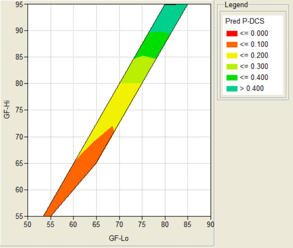
SAUL is a probabilistic model. This means that rather than telling you if a certain dive is ok from the perspective of the model or telling you the fastest way out of the water that is still considered save by the model (like our traditional models like Bühlmann or VPM-B, possibly enriched by adjustable fudge factors like gradient factors or conservatism) a probabilistic model will give you a probability for a dive to result in decompression illness.
In the case auf SAUL, these probabilities are based on series of empirical tests, where a (large) number of divers followed a given deco schedule and you count the number of DCS cases. This is not any different from any other empirical study.
What I want to discuss in this post is how to design a study to establish the fact that “the accident probability for this given profile is less than some probability p”. So, this post is about the statistics of setting up such a study. Please be aware that I am by no means an expert on statistics, this is all pretty much home grown (I did some googling but could not easily find a good reference for the whole story), so chances are even higher than otherwise that I am completely wrong. But in this case, please teach me!
Note that I want to establish the safety of a plan (as a bound on the probability of injury) but simply do a number N of dives, count the number a of accidents and then claim that the probability is a/N. Rather, I want a confidence interval. To be specific, I want that the probability of “the accident probability (or rate) is higher than one in a thousand” is less than 5% (that seems to be a pretty common number as 95% contains two standard deviations for a normal distribution).
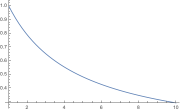
So for example, we could do N dives and hope to find no accident. The probability that happens by chance is
\((1-p)^N\)if p is the accident probability. So this should be less or equal than c=0.05. When we solve that for N we find
\(N=\frac{\ln c}{\ln(1-p)}\)and as we expect p to be pretty small, we can chop of the Maclaurin series after the first term and thanks to ln(0.05) being almost -3 write
\(N\approx 3/p.\)So, to establish a probability of 1/1000 we would have to conduct 3000 dives in our study. So, let’s apply for funding.
The problem is only, that we won’t get that funding. Because we will be able to show our hypothesis only in the case of no accident. But we just computed that that chance is 5%. So in 95% of studies conducted like this, the result will only be inconclusive. We have to do better.
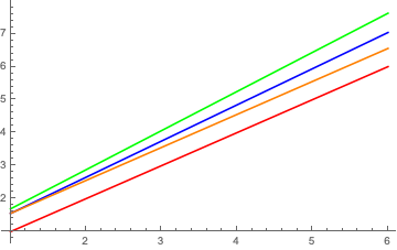
Doing better might mean, not being that ambitious, but aiming for a not so strong hypothesis. We could try to show that the probability is only smaller than 1/500. Then we would do 1500 dives with an expected number of accidents (as we believe the true probability is still 1/1000) of 1.5.
Or we actually believe that the true probability is actually 1/2000. And then we could no more dives, such that the allowed accident number can be higher still leading to a 1/1000 bound on the probability.
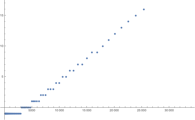
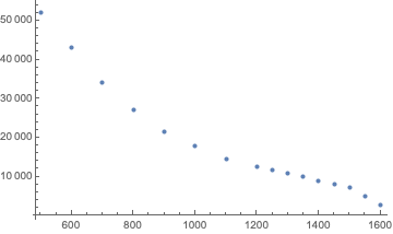
And for these numbers, we can then compute the chance of having a successful study (i.e. one where the number of DCS cases is indeed small enough) when the true probability of DCS for this dive is actually 1/2000:

Two things I found remarkable: You actually need of the order of 10,000 dives to have a 50:50 chance for a significant study establishing an accident probability of at most 0.001. I have been using this probability as I think an accident rate of 1 in 1000 is what is generally accepted at least in recreational diving (would it be significantly higher, the whole industry would quickly go down the drain thanks to people suing others for liability). But studies with 10,000 dives are totally unrealistic as far too expensive. This is why you want to conduct studies with much higher accident rates, so you can establish those with much fewer dives. A famous example being the NEDU deep stop study that put their divers under severe stress (cold, exercise etc) to drive up the accident rate. And they were criticised for these “totally irrelevant to actual diving” conditions in particular by those being in favour of deep stops. Only that with “realistic” dives, it would be very hard and expensive to see a significant effect.
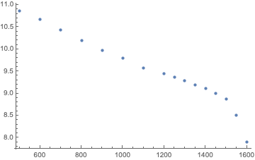
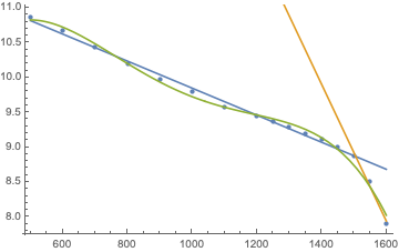
The other lesson is more formal: in a range where the allowed number of deco cases is constant, the chance for a successful study decreases with increasing N. This I did not expect but it is quite obvious: With every additional dive, you increase the chance of having another accident that kills the study. So, if you design such a study, you should pick N just slightly bigger than one of the jumps of allowed DCS cases.
As always, I made my mathematica notebook for these calculations available.